Università degli Studi di Verona
DEPARTMENT OF COMPUTER SCIENCE
Master Degree in Mathematics
Data-driven modelling and calibration of multi-agent systems
| Candidate: Andrea Mortaro |
Supervisor: Prof. Dott. Giacomo Albi |
Introduction
We aim to analyze interaction dynamics using data-driven techniques. The emphasis is on:
- Discrete-to-continuum transition in traffic modelling;
- Neural networks for modelling interactions with data.
Traffic models
Traffic models
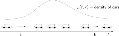
Our focus lies in uncovering the underlying connection in traffic modelling between:
- Macroscopic models, as the Lighthill–Whitham–Richards (LWR) model;
- Microscopic models, as the Follow-The-Leader-type (FTL) models.
Traffic models
Macroscopic models
Traffic models
Macroscopic models
\begin{equation*} \rho_{t} + \left( f(\rho) \right)_{x} = 0, \quad t>0,\, x \in \mathbb{R} \end{equation*}
Traffic models
Microscopic models
Traffic models
Microscopic models
\begin{equation*} \left\{ \begin{aligned} & \dot{x}_{n} = v_{max} \\ & \dot{x}_{i} = v \left( \dfrac{ \ell }{ x_{i+1} - x_{i} } \right), \quad &&i = 1,... , n-1. \end{aligned} \right. \end{equation*}
Traffic models
Traffic models
Theoretical analysis
Traffic models
Theoretical analysis
Consider the Cauchy problem: \begin{equation} \label{cauchy} \left\{ \begin{aligned} & \rho_{t} + \left(f(\rho)\right)_{x} = 0, \quad &&(t,x) \in (0, +\infty) \times \mathbb{R}, \\ & \rho(0,x) = \bar{\rho}(x), \quad &&x \in \mathbb{R}, \end{aligned} \right. \end{equation}
where $f(\rho)\ \dot{=}\ \rho\ v(\rho)$.
Traffic models
Theoretical analysis
Assume that $\bar{\rho}$ and $v:\mathbb{R}_{+}\rightarrow\mathbb{R}$ satisfy: \begin{equation} \label{hp:rho} \bar{\rho} \in \mathcal{L}^\infty(\mathbb{R}) \cap \mathcal{L}^1(\mathbb{R}),\quad \bar{\rho} \geq 0, \end{equation} \begin{equation} \label{hp:v} v \in \mathcal{C}^1(\mathbb{R}_{+}),\quad v'(\rho) < 0\ for\ \rho > 0. \end{equation}
Sometimes, we require extra-assumptions: \begin{equation} \label{addhp:rho} \bar{\rho} \in \mathcal{BV}(\mathbb{R}), \end{equation} \begin{equation} \label{addhp:v} \mathbb{R}^{+} \ni \rho \mapsto \rho\ v'(\rho) \in \mathbb{R}^{-}. \end{equation}
Traffic models
Theoretical analysis
Definition 1 (Entropy solution). Let the initial datum $\bar{\rho}$ satisfy \eqref{hp:rho}. A weak solution $\rho \in \mathcal{L}^\infty(\mathbb{R})$ to the Cauchy problem \eqref{cauchy} is called entropy solution to the Cauchy problem if:
\begin{equation*} \iint\limits_{\mathbb{R}^+ \times \mathbb{R}} \bigg[ |\rho(t,x) - k|\varphi_{t}(t,x)\ +\ \text{sign}(\rho(t,x) - k) \left[ f(\rho(t,x)) - f(k)\right]\varphi_{x}(t,x)\bigg] dx\ dt\ \geq 0 \end{equation*}
for all $\varphi \in \mathcal{C}_{c}^\infty((0, +\infty) \times \mathbb{R})$ and for all $k \geq 0$.
Traffic models
Theoretical analysis
Theorem 1 (Existance and uniqueness). Assume that \eqref{hp:rho} and \eqref{hp:v} are satisfied. Then there exists a unique entropy solution according to Definition 1.
Theorem 2 (Convergence). Assume that \eqref{hp:rho} and \eqref{hp:v} are satisfied. Moreover, assume that at least one of the two conditions \eqref{addhp:rho} and \eqref{addhp:v} are satisfied. Then $\rho^{n}$ converges (up to a subsequence) almost everywhere and in $\mathcal{L}^{1}_{loc}$ on $\mathbb{R}_{+} \times \mathbb{R}$ to the unique entropy solution $\rho$ to the Cauchy problem \eqref{cauchy}, according to Definition 1.
Traffic models
Approximating Scheme
Traffic models
Approximating Scheme
For $n \in \mathbb{N}$ large, we set $\ell_{n} \dot{=}\ \frac{1}{n}$ and we define:
\begin{equation*} \bar{x}^{n}_{1}\ \dot{=}\ \text{sup} \bigg\{ x \in \mathbb{R}: \int_{-\infty}^{x} \bar{\rho}(x)\ dx\ < \ell_{n} \bigg\}, \end{equation*} \begin{equation*} \bar{x}^{n}_{i}\ \dot{=}\ \text{sup} \bigg\{ x \in \mathbb{R}: \int_{\bar{x}^{n}_{i-1}}^{x} \bar{\rho}(x)\ dx\ < \ell_{n} \bigg\} \; \forall i\ \in\ \{2,...,n-1\}. \end{equation*}
Traffic models
Approximating Scheme
Let the particles $\{\bar{x}^{n}_{i}\}^{n-1}_{i=1}$ evolve according to the Follow-The-Leader system of ODEs: \begin{equation*} \left\{ \begin{aligned} & \dot{x}^{n}_{i}(t) = v(R^{n}_{i}(t)),\quad\ &i \in \{1,...,n-2\},\\ & \dot{x}^{n}_{n-1}(t) = v_{max}, \\ & x^{n}_{i}(0) = \bar{x}^{n}_{i},\quad\ &i \in \{1,...,n-1\}, \\ \end{aligned} \right. \end{equation*} where $R^{n}_{i}(t)\ \dot{=}\ \frac{\ell_{n}}{x^{n}_{i+1}(t)-x^{n}_{i}(t)}$.
Traffic models
Approximating Scheme
Set two artificial particles for all $t \geq 0$ as: \begin{equation*} x^{n}_{0}(t)\ \dot{=}\ 2x^{n}_{1}(t) - x^{n}_{2}(t),\qquad x^{n}_{n}(t)\ \dot{=}\ 2x^{n}_{n-1}(t) - x^{n}_{n-2}(t), \end{equation*} and let \begin{equation*} R^{n}_{0}(t)\ \dot{=}\ R^{n}_{1}(t), \qquad R^{n}_{n}(t)\ \dot{=}\ R^{n}_{n-1}(t). \end{equation*}
Traffic models
Approximating Scheme
\begin{equation} \label{density:def} \begin{aligned} \rho^{n}(t,x)\ \dot{=}&\ \sum_{i=0}^{n-1} R^{n}_{i}(t)\ \unicode{x1D7D9}_{[x^{n}_{i}(t),x^{n}_{i+1}(t)]}(x)\\ =&\ \sum_{i=0}^{n-1} \frac{\ell_{n}}{x^{n}_{i+1}(t)-x^{n}_{i}(t)}\ \unicode{x1D7D9}_{[x^{n}_{i}(t),x^{n}_{i+1}(t)]}(x), \end{aligned} \end{equation}
Traffic models
Sketch of the proof
Traffic models
Sketch of the proof
Theorem 2 (Convergence). Assume that \eqref{hp:rho} and \eqref{hp:v} are satisfied. Moreover, assume that at least one of the two conditions \eqref{addhp:rho} and \eqref{addhp:v} are satisfied. Then $\rho^{n}$ converges (up to a subsequence) almost everywhere and in $\mathcal{L}^{1}_{loc}$ on $\mathbb{R}_{+} \times \mathbb{R}$ to the unique entropy solution $\rho$ to the Cauchy problem \eqref{cauchy}, according to Definition 1.
Traffic models
Sketch of the proof: compactness
Traffic models
Sketch of the proof: compactness
First way: A uniform $\mathcal{BV}$ contraction property for $\rho^{n}$, which requires $\mathcal{BV}$ initial data \eqref{addhp:rho}.
Second way: Use the discrete Oleinik-type inequality, which doesn't require the extra-assumption \eqref{addhp:rho} on $\bar{\rho}$, but only \eqref{addhp:v} on $v$.
Third way: To achieve strong $\mathcal{L}^{1}$ compactness we consider 1-Wasserstein distance.
Traffic models
Sketch of the proof: compactness
Theorem 3 (Generalised Aubin-Lions lemma). Let $\,T > 0, \,a,b \in \mathbb{R}, a < b$ and $v$ satisfy \eqref{hp:v}. Let $\rho^{n}$ be a sequence in $\mathcal{L}^{\infty} \left( (0,T);\ \mathcal{L}^{1}(\mathbb{R}) \right)$ with: \begin{equation*} \rho^{n} (t, \cdot) \geq 0, \quad \| \rho^{n} (t, \cdot) \|_{\mathcal{L}^{1}(\mathbb{R})} = 1 \; \forall n \in \mathbb{N}, \; \forall t \in \left[ 0,T \right]. \end{equation*} Assume further that:
- $\sup_{n \in \mathbb{N}} \left[ \int_{0}^{T} \big[ \| v(\rho^{n}(t, \cdot)) \|_{\mathcal{L}^{1} ( \left[ a,b \right] ) } + TV \left( v(\rho^{n}(t,\cdot));\ \left[ a,b \right] \right) \big] dt \right] < +\infty,$
- $\exists\, C>0$ independent of $n$ such that \begin{equation*} W_{1} (\rho^{n}(t,\cdot), \rho^{n}(s,\cdot) ) \leq C |t-s| \quad \forall \text{t,s} \in (0,T). \end{equation*}
Then $\rho^{n}$ is strongly relatively compact in $\mathcal{L}^{1} \left( \left[ 0,T \right] \times \left[ a,b \right]\right)$.
Traffic models
Sketch of the proof: convergence
Traffic models
Sketch of the proof: convergence
Once gained strong $\mathcal{L}^{1}$ compactness and by passing from $\left[ \delta, T \right]$ to $( 0,T )$, one can show that $\rho^{n}$ admits a converging subsequence a.e. in $\mathcal{L}^{1} \left( \left( 0,T \right) \times \mathbb{R} \right)$. Denote $\rho$ such limit.
Traffic models
Sketch of the proof: convergence
Step 1: $\rho$ is a weak solution to \eqref{cauchy}. Let $\varphi \in \text{C}^{\infty}_{\text{c}} \left( \mathbb{R}_{+} \times \mathbb{R} \right)$. \begin{align*} \def\avint{\mathop{\,\rlap{-}\!\!\int}\nolimits} & \iint_{\mathbb{R}_{+} \times \mathbb{R}} \Big[ \rho^{n} (t,x)\, \varphi_{t} \left( t, x \right) + \rho^{n}(t,x)\, v( \rho^{n}(t,x) )\, \varphi_{x} \left( t,x \right) \Big] dx\, dt\\ & \leq \ 2 \ell_{n} \| \varphi (0,\cdot) \|_{\mathcal{L}^{\infty}(\mathbb{R})} + \sum_{i=0}^{n-1} \left| \int_{\bar{x}_{i}^{n}}^{\bar{x}_{i+1}^{n}} \bar{\rho} (x) \left[ \varphi (0,x) - \avint_{\bar{x}_{i}^{n}}^{\bar{x}_{i+1}^{n}} \varphi (0,y)\, dy \right] dx \right| \end{align*}
Traffic models
Sketch of the proof: convergence
Step 2: $\rho$ satisfies the entropy inequality in Definition 1. Let $\varphi \in \text{C}^{\infty}_{\text{c}} \left( \left( 0,+\infty \right) \times \mathbb{R} \right)$ with $\varphi \geq 0$ and $k \geq 0$.
\begin{align*} & \iint\limits_{\mathbb{R}^{+} \times \mathbb{R}} \bigg[ |\rho(t,x) - k| \varphi_{t}(t,x)\ +\ \text{sign}(\rho(t,x) - k) \left[ f(\rho(t,x)) - f(k)\right]\varphi_{x}(t,x)\bigg] dx \, dt \\ & =\ k \int_{\mathbb{R}^{+}} \Big[ \big[ v(k) - \dot{x}_{0}^{n}(t) \big] \varphi(t, x_{0}^{n}(t)) + \big[ v(k) - \dot{x}_{n}^{n}(t) \big] \varphi(t, x_{n}^{n}(t)) \Big] dt\\ & \hspace{20pt} + \sum_{i=0}^{n-1} \int_{\mathbb{R}^{+}} \text{sign} \left( R_{i}^{n}(t) - k \right) \Bigg[ - \dot{R}_{i}^{n} (t) \left( \int_{x_{i}^{n}(t)}^{x_{i+1}^{n}(t)} \varphi (t,x) dx \right)\\ & \hspace{20pt} - \Big[ R_{i}^{n} (t) \left[ \dot{x}_{i+1}^{n}(t) - v(R_{i}^{n} (t)) \right] - k \left[ \dot{x}_{i+1}^{n}(t) - v(k) \right] \Big] \varphi (t, x_{i+1}^{n}(t))\\ & \hspace{20pt} + \Big[ R_{i}^{n} (t) \left[ \dot{x}_{i}^{n}(t) - v(R_{i}^{n} (t)) \right] - k \left[ \dot{x}_{i}^{n}(t) - v(k) \right] \Big] \varphi (t, x_{i}^{n}(t)) \Bigg] dt.\\ \end{align*}
Traffic models
Traffic Scenario
Traffic models
Traffic Scenario
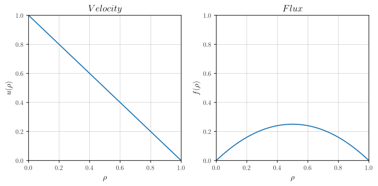
Assume $f (\rho) = \rho\ v(\rho)$ and consider $v(\rho) = 1-\rho$ with speed limit $v_{max}=1$ in: \begin{equation*} \rho_{t} + \left( f (\rho) \right)_{x} = 0, \quad t>0,\, x \in \mathbb{R}. \end{equation*}
Traffic models
Traffic Scenario
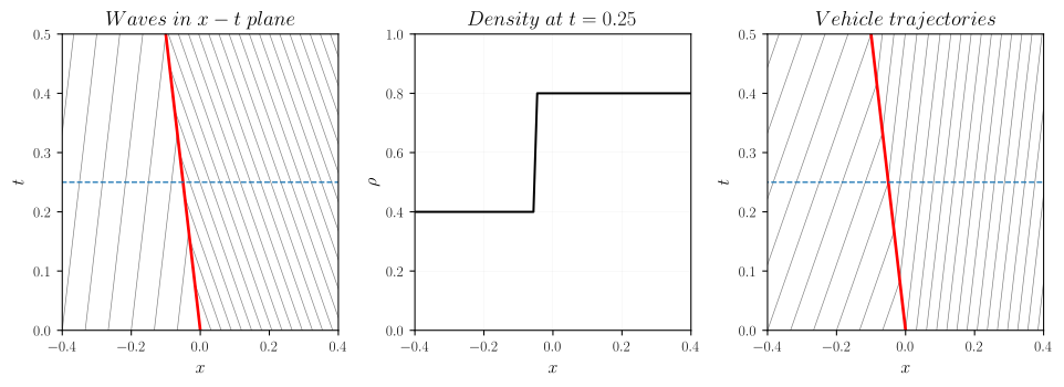
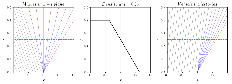
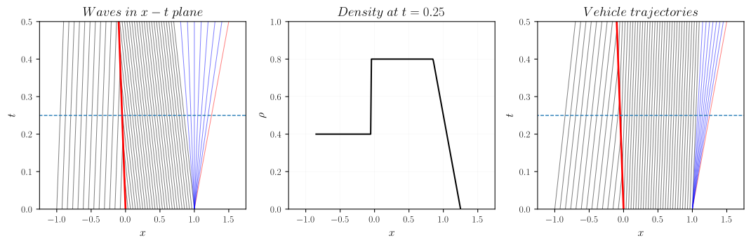
Consider the Riemann problem for the LWR equation \begin{equation} \label{cauchy:trafficflow} \left\{ \begin{aligned} & \rho_{t} + \left(f(\rho)\right)_{x} = 0, \quad &&(t,x) \in (0, +\infty) \times \mathbb{R}, \\ & \rho(0,x) = \bar{\rho}(x) \quad &&x \in \mathbb{R}, \end{aligned} \right. \end{equation} equipped with the initial condition: \begin{equation} \bar{\rho}(x) = \begin{cases} 0.4 & -1 \leq x \leq 0, \\ 0.8 & 0 < x \leq 1, \\ 0 & otherwise. \end{cases} \label{rhozero} \end{equation}
Traffic models
Traffic Scenario
Traffic jam. At $x=0$, traffic approaches a congested area, since $\rho$ is close to $1$. This corresponds to the discontinuity (or shock wave) moving to the left.
Traffic models
Traffic Scenario
Green light. When the light at $x=1$ changes at time $t=0$, there is no traffic after the light. Therefore cars spread out and it appears a rarefaction wave.
Traffic models
Traffic Scenario
Traffic models
Traffic Scenario
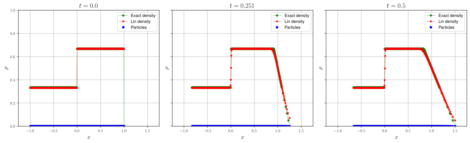
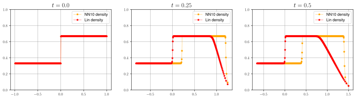
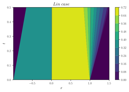
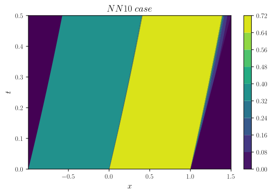
Redefine the initial datum $\bar{\rho}$ as: \begin{equation} \label{rhozero2} \bar{\rho}(x) = \begin{cases} 0.\bar{3} & -1 \leq x \leq 0, \\ 0.\bar{6} & 0 < x \leq 1, \\ 0 & \text{otherwise}. \end{cases} \end{equation}
Traffic models
Traffic Scenario
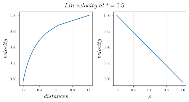
Evolution of $\rho^{n}$ with initial datum \eqref{rhozero2}. We take $N = 400$, final time $T = 0.5$ and $(L,v_0) = (0.0025,1)$.
Traffic models
Traffic Scenario
Model Calibration with Data
Model Calibration with Data
Optimal Control framework
Model Calibration with Data
Optimal Control framework
Consider the cost functional: \begin{equation*} J \left( x(u);z \right) \, =\, \dfrac{1}{2} \int_{0}^{T} \| z(t) - x(t) \|^{2} dt \, =\, \dfrac{1}{2} \| z(t) - x(t) \|^{2}_{\mathcal{L}^{2}(\mathbb{R})}. \end{equation*} and the dynamics is given by: \begin{equation} \label{x:dyn} \frac{ d }{ dt } x_{i} \, =\, \sum_{j = 1}^{N} W_{u}^{i,j} (x_{j} - x_{i}), \quad x_{i}(0) = z_{0}^{i}, \qquad i = 1, ..., N. \end{equation}
Model Calibration with Data
Optimal Control framework
Problem 1 . Find $\bar{u} \in \mathcal{U}_{ad} := \left[ -1, 1 \right]^{K}$ such that \begin{equation*} J \left( x(u);z \right) \, =\, \min_{u\, \in\, \mathcal{U}_{ad}} J \left( x(u); z \right) \quad \text{subject to \eqref{x:dyn}}, \end{equation*}
Model Calibration with Data
Data-driven parameter estimation
Model Calibration with Data
Data-driven parameter estimation
Traffic dynamic with LWR-model
Let $x_{i}(t)$ denote the position of the $i$-th car at time $t \in \left[ 0, T\right]$. Then:
\begin{equation} \label{td:lwr} \left\{ \begin{aligned} & \dot{x}_{i}(t)\, =\, W_{u}^{i,i+1}\, \bigg( \dfrac{ x_{i+1}(t) - x_{i}(t)}{L} \bigg), \quad i \in 1,... , N-1, \\ & \dot{x}_{N}(t)\, =\, v_{0}, \end{aligned} \right. \end{equation}
For $z > 0$, we model the velocity function as:
- $ W_{u}^{i,i+1} (z) = v_{0} \left(1 - \dfrac{1}{z} \right)$ for the linear case.
- $ W_{u}^{i,i+1} (z) = v_{0}\, \text{log}(z)$ for the logarithmic case;
Model Calibration with Data
Data-driven parameter estimation
Traffic dynamic with artificial neural network
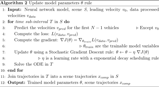
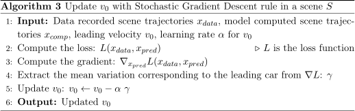
Consider $W_{u}$ as the output of a neural network parameterized by $u$:
\begin{equation} \label{td:ann} \left\{ \begin{aligned} & \dot{x}_{i}(t)\, =\, W_{u}^{i,i+1}\, \big( x_{i+1}(t) - x_{i}(t) \big), \quad i \in 1,... , N-1, \\[1ex] & \dot{x}_{N}(t)\, =\, v_{0}. \end{aligned} \right. \end{equation}
where $u = \left(v_0, u_{Net}\right)$.
Model Calibration with Data
Data-driven parameter estimation
The task of the parameter identification is to estimate:
- $u = \left( L, v_{0} \right) \in \mathbb{R}^{2}$ in the LWR traffic model
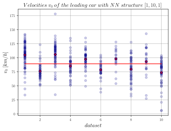
- $u = \left(v_0, u_{Net}\right) \in \mathbb{R}^{2}$ in the artificial neural network-driven traffic model
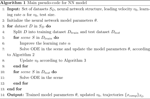
 Real data provided by the ESIMAS project.
Model Calibration with Data
Data-driven parameter estimation
Model Calibration with Data
Data-driven parameter estimation
Model Calibration with Data
Data-driven parameter estimation
Model Calibration with Data
Traffic Models Training Results
Model Calibration with Data
Traffic Models Training Results
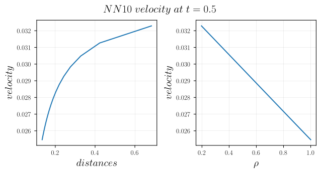
Initial values are $v_{0} = 30~m/s$ and $L = 5~m$. The weights are initialized in $\, \mathcal{U} \left( \left[ -1, 1 \right] \right)$.
Model Calibration with Data
Traffic Models Training Results
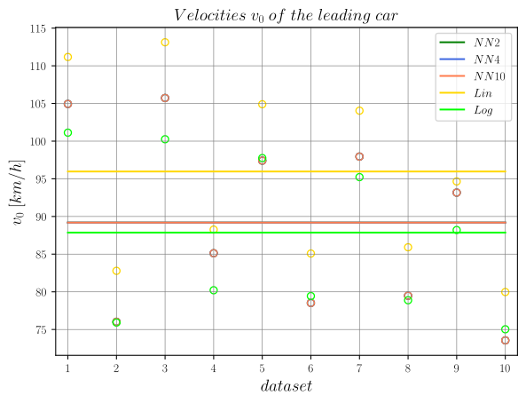
Initial values are $v_{0} = 30~m/s$ and $L = 5~m$.
Model Calibration with Data
Traffic Models Training Results
Car lengths estimated using LWR-model with linear and logarithmic velocity, setting $L_{min} = 2~m$ as the lower bound.

Model Calibration with Data
Traffic Models Training Results
Model Calibration with Data
Traffic Models Training Results
Model Calibration with Data
Traffic Models Training Results
|
|
Conclusions and Future Developments
The aims of this study were:
- Analysis of the discrete-to-continuum transition in traffic models;
- Application of Neural Network-driven models to describe traffic dynamics scenarios.
Conclusions and Future Developments
Immediate developments of this work may involve:
- Incorporating physics into Neural Networks via Physics-Informed Neural Networks (PINNs);
- Enhancing Neural Network architecture with Recurrent Neural Networks (RNNs).
Thank you for your attention!