- Welcome to Congo! :tada:/
- Posts/
- Some exercise about Statistical Learning/
- SL2: Analysis of Prostate Cancer dataset - linear regression model/
SL2: Analysis of Prostate Cancer dataset - linear regression model
Table of Contents
Aim of the analysis
We want to examinate correlation between the level of prostate-specific antigen and a number of clinical parameters in men, who are about to receive a prostatectomy.
# data analysis and wrangling
import numpy as np # linear algebra
import pandas as pd # data processing, CSV file I/O (e.g. pd.read_csv)
# import random as rnd

# visualization
import seaborn as sns
import matplotlib.pyplot as plt
# %matplotlib inline

# machine learning
from sklearn.linear_model import LinearRegression
from sklearn.metrics import r2_score
from sklearn.metrics import mean_squared_error


import statsmodels.api as sm

from IPython.display import Image # to visualize images
from tabulate import tabulate # to create tables

import os
for dirname, _, filenames in os.walk('/kaggle/input'):
    for filename in filenames:
        print(os.path.join(dirname, filename))
/kaggle/input/prostate-data/prostate.data
/kaggle/input/prostate-data/tab.png
/kaggle/input/prostate-data/tab2.png
1. Open the webpage of the book “The Elements of Statistical Learning”, go to the “Data” section and download the info and data files for the dataset called Prostate
2. Open the file `prostate.info.txt`
Hint: please, refer also to Section 3.2.1 (page 49) of the book “The Elements of Statistical Learning” to gather this information
How many predictors are present in the dataset? What are those names?
There are 8 predictors:
1. lcavol (log cancer volume)
2. lweight (log prostate weight)
3. age
4. lbph (log of the amount of benign prostatic hyperplasia)
5. svi (seminal veiscle invasion)
6. lcp (log of capsular penetration)
7. gleason (Gleason score)
8. pgg45 (percent of Gleason scores 4 or 5)How many responses are present in the dataset? What are their names?
There is one response: 1. lpsa (log of prostate-specific antigen)
How did the authors split the dataset in training and test set?
They randomly split the dataset (containing 97 observations, in
prostate.data) into a training set of size 67 and a test set of size 30.
In the fileprostate.datathere is a columntrainwhich is of boolean type in order to distinguish if an observation is used (T) or not (F) to train the model.
3. Open the file `prostate.data` by a text editor or a spreadsheet and have a quick look at the data
- How many observations are present?
There are 97 observations in total.
- Which is the symbol used to separate the columns?
To separate the columns there is the escape character
\ttab.
4. Open Kaggle, generate a new kernel and give it the name “SL_EX2_ProstateCancer_Surname”
5. Add the dataset `prostate.data` to the kernel
- Hint: See the Add Dataset button on the right
- Hint: use import option “Convert tabular files to csv”
6. Run the first cell of the kernel to check if the data file is present in folder ../input
7. Add to the first cell new lines to load the following libraries: seaborn, matplotlib.pyplot, sklearn.linear_model.LinearRegression
pandas.8. Add a Markdown cell on top of the notebook, copy and paste in it the text of this exercise and provide in the same cell the answers to the questions that you get step-by-step.
9. Load the Prostate Cancer dataset into a Pandas DataFrame variable called "data"
- How can you say Python to use the right separator between columns?
I need to specify
sep='\tintoread_csvmethod in order to load the dataset.
Data acquisition #
# Load the Prostate Cancer dataset
data = pd.read_csv('../input/prostate-data/prostate.data',sep='\t')
# data.info() # to check if it is correct
10. Display the number of rows and columns of variable data
[num_rows,num_columns]=data.shape;

print(f"The number of rows is {num_rows} and the number of columns is {num_columns}.")
The number of rows is 97 and the number of columns is 11.
11. Show the first 5 rows of the dataset
data.head(5)
| Unnamed: 0 | lcavol | lweight | age | lbph | svi | lcp | gleason | pgg45 | lpsa | train | |
|---|---|---|---|---|---|---|---|---|---|---|---|
| 0 | 1 | -0.579818 | 2.769459 | 50 | -1.386294 | 0 | -1.386294 | 6 | 0 | -0.430783 | T |
| 1 | 2 | -0.994252 | 3.319626 | 58 | -1.386294 | 0 | -1.386294 | 6 | 0 | -0.162519 | T |
| 2 | 3 | -0.510826 | 2.691243 | 74 | -1.386294 | 0 | -1.386294 | 7 | 20 | -0.162519 | T |
| 3 | 4 | -1.203973 | 3.282789 | 58 | -1.386294 | 0 | -1.386294 | 6 | 0 | -0.162519 | T |
| 4 | 5 | 0.751416 | 3.432373 | 62 | -1.386294 | 0 | -1.386294 | 6 | 0 | 0.371564 | T |
12. Remove the first column of the dataset which contains observation indices
print("* Before to drop the first column:")
data.info()
#data1 = data1.drop(columns='Unnamed: 0')
#data1 = data1.drop(labels=['Unnamed: 0'],axis=1)

print("\n* After having dropped the first column:")
data = data.drop(data.columns[0],axis=1) # without specifying the name of the variable (axis=0 indicates rows, axis=1 indicates columns)
data.info()

data['train'].value_counts()
* Before to drop the first column:

<class 'pandas.core.frame.DataFrame'>
RangeIndex: 97 entries, 0 to 96
Data columns (total 11 columns):
 #   Column      Non-Null Count  Dtype
---  ------      --------------  -----
 0   Unnamed: 0  97 non-null     int64
 1   lcavol      97 non-null     float64
 2   lweight     97 non-null     float64
 3   age         97 non-null     int64
 4   lbph        97 non-null     float64
 5   svi         97 non-null     int64
 6   lcp         97 non-null     float64
 7   gleason     97 non-null     int64
 8   pgg45       97 non-null     int64
 9   lpsa        97 non-null     float64
 10  train       97 non-null     object
dtypes: float64(5), int64(5), object(1)
memory usage: 8.5+ KB


* After having dropped the first column:

<class 'pandas.core.frame.DataFrame'>
RangeIndex: 97 entries, 0 to 96
Data columns (total 10 columns):
 #   Column   Non-Null Count  Dtype
---  ------   --------------  -----
 0   lcavol   97 non-null     float64
 1   lweight  97 non-null     float64
 2   age      97 non-null     int64
 3   lbph     97 non-null     float64
 4   svi      97 non-null     int64
 5   lcp      97 non-null     float64
 6   gleason  97 non-null     int64
 7   pgg45    97 non-null     int64
 8   lpsa     97 non-null     float64
 9   train    97 non-null     object
dtypes: float64(5), int64(4), object(1)
memory usage: 7.7+ KB


T    67
F    30
Name: train, dtype: int64
13. Save column train in a new variable called "train" and having type `Series` (the Pandas data structure used to represent DataFrame columns), then drop the column train from the data DataFrame
# Save "train" column in a Pandas Series variable
train = data['train']
# train = pd.Series(data['train'])

# Drop "train" variable from data
data = data.drop(columns=['train'])
14. Save column lpsa in a new variable called "lpsa" and having type `Series` (the Pandas data structure used to represent DataFrame columns), then drop the column lpsa from the data DataFrame and save the result in a new DataFrame called predictors
- How many predictors are available?
There are 8 predictors available for each one of the 97 observations.
# Save "lpsa" column in a Pandas Series variable
lpsa = data['lpsa']
# lpsa = pd.Series(data['lpsa'])

# Drop "train" variable from data
data = data.drop(columns=['lpsa'])
predictors = data
predictors.info()
<class 'pandas.core.frame.DataFrame'>
RangeIndex: 97 entries, 0 to 96
Data columns (total 8 columns):
 #   Column   Non-Null Count  Dtype
---  ------   --------------  -----
 0   lcavol   97 non-null     float64
 1   lweight  97 non-null     float64
 2   age      97 non-null     int64
 3   lbph     97 non-null     float64
 4   svi      97 non-null     int64
 5   lcp      97 non-null     float64
 6   gleason  97 non-null     int64
 7   pgg45    97 non-null     int64
dtypes: float64(4), int64(4)
memory usage: 6.2 KB
15. Check the presence of missing values in the `data` variable
Since all the columns are numerical variables, we have not to distinguish variables between numerical and categorical kind.- How many missing values are there? In which columns?
We have no missing values.
- Which types do the variable have?
lcavol,lweight,lbphandlcpare float64, whileage,svi,gleasonandpgg45are int64
print("For each variable in data, we have no missing values:\n\n",data.isna().sum())
For each variable in data, we have no missing values:

lcavol     0
lweight    0
age        0
lbph       0
svi        0
lcp        0
gleason    0
pgg45      0
dtype: int64
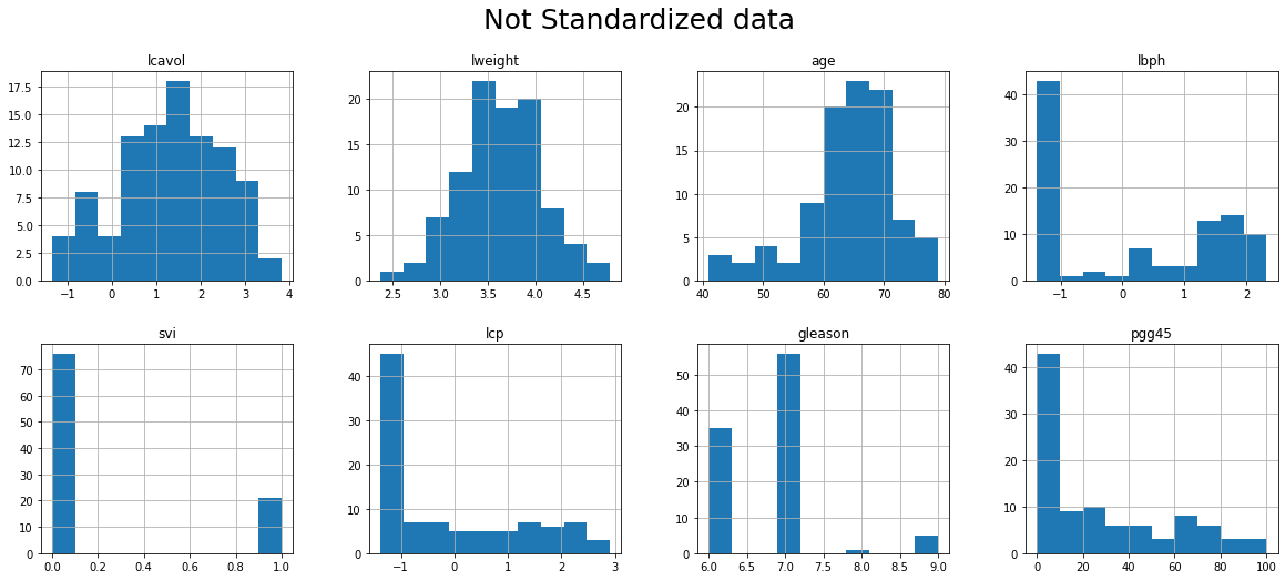
16. Show histograms of all variables in a single figure
- Use argument figsize to enlarge the figure if needed
fig = plt.figure()

predictors.hist(grid=True, figsize=(20,8), layout = (2,4))

fig.tight_layout()
plt.suptitle("Not Standardized data", fontsize=25)

fig.show()
<Figure size 432x288 with 0 Axes>
17. Show the basic statistics (min, max, mean, quartiles, etc. for each variable) in data
data.describe()
| lcavol | lweight | age | lbph | svi | lcp | gleason | pgg45 | |
|---|---|---|---|---|---|---|---|---|
| count | 97.000000 | 97.000000 | 97.000000 | 97.000000 | 97.000000 | 97.000000 | 97.000000 | 97.000000 |
| mean | 1.350010 | 3.628943 | 63.865979 | 0.100356 | 0.216495 | -0.179366 | 6.752577 | 24.381443 |
| std | 1.178625 | 0.428411 | 7.445117 | 1.450807 | 0.413995 | 1.398250 | 0.722134 | 28.204035 |
| min | -1.347074 | 2.374906 | 41.000000 | -1.386294 | 0.000000 | -1.386294 | 6.000000 | 0.000000 |
| 25% | 0.512824 | 3.375880 | 60.000000 | -1.386294 | 0.000000 | -1.386294 | 6.000000 | 0.000000 |
| 50% | 1.446919 | 3.623007 | 65.000000 | 0.300105 | 0.000000 | -0.798508 | 7.000000 | 15.000000 |
| 75% | 2.127041 | 3.876396 | 68.000000 | 1.558145 | 0.000000 | 1.178655 | 7.000000 | 40.000000 |
| max | 3.821004 | 4.780383 | 79.000000 | 2.326302 | 1.000000 | 2.904165 | 9.000000 | 100.000000 |
18. Generate a new DataFrame called dataTrain and containing only the rows of data in which the train variable has value “T”
- Hint: use the loc attribute of DataFrame to access a groups of rows and columns by label(s) or boolean arrays
- How many rows and columns does dataTrain have?
dataTrain = data.loc[train == 'T'] # Obviously, len(idx)==len(dataTrain) is True!

# # Alternative way:
# # 1. Get the indexes corresponding to train ==  'T'
# idxTrain = train.loc[train == 'T'].index.tolist()
# # 2. Access to interesting rows with .iloc()
# dataTrain = data.iloc[idxTrain]

print(f"dataTrain contains {dataTrain.shape[0]} rows and {dataTrain.shape[1]} columns.")
dataTrain contains 67 rows and 8 columns.
19. Generate a new DataFrame called dataTest and containing only the rows of data in which the train variable has value “F”
- How many rows and columns does dataTest have?
dataTest = data.loc[train == 'F']
20. Generate a new Series called lpsaTrain and containing only the values of variable lpsa in which the train variable has value “T”
- How many valuses does lpsaTrain have?
# Create a new Series variable
lpsaTrain = lpsa.loc[train == 'T']

# # Another way to define it
# data_all = pd.read_csv('../input/prostate-data/prostate.data',sep='\t')
# lpsaTrain = data_all.loc[train == 'T']['lpsa']

# # To check if it is correct:
# idxTrain = train.loc[train == 'T'].index.tolist()
# lpsaTrain == lpsa.iloc[idxTrain]

print(f"lpsaTrain has {lpsaTrain.shape[0]} values.")
lpsaTrain has 67 values.
21. Generate a new Series called lpsaTest and containing only the values of variable lpsa in which the train variable has value “F”
- How many valuses does lpsaTest have?
lpsaTest = lpsa.loc[train == 'F']

# # To check if it is correct:
# len(lpsaTest) == len(data)-len(lpsaTrain)

print(f"lpsaTrain has {lpsaTest.shape[0]} values.")
lpsaTrain has 30 values.
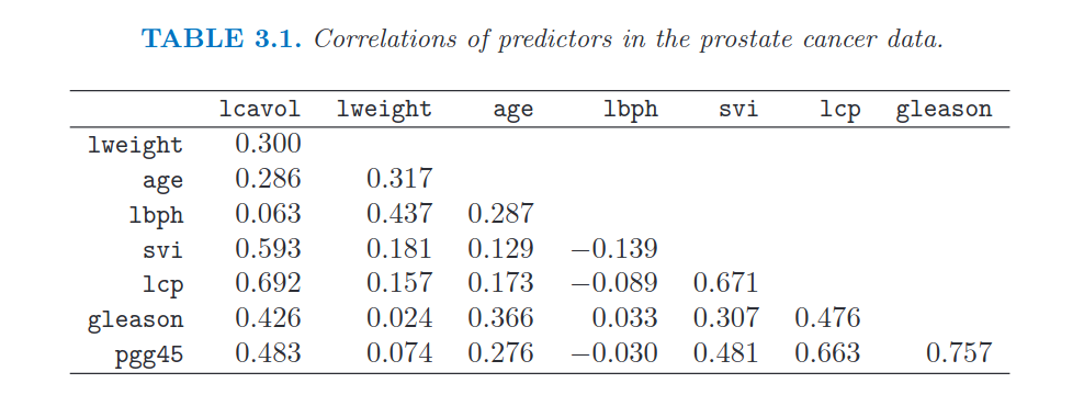
22. Show the correlation matrix among all the variables in dataTrain
- Hint: use the correct method in DataFrame
- Hint: check if the values in the matrix correspond to those in Table 3.1 of the book
# Create correlation matrix
corrM = dataTrain.corr().round(decimals = 3) # As in the book, I plot values up to 3 decimals

# Display only the lower diagonal correlation matrix
lowerM = np.tril(np.ones(corrM.shape), k=-1) # Lower matrix of ones. (for k=0 I include also the main diagonal)
cond = lowerM.astype(bool) # Create a matrix of false, except in lowerM
corrM = corrM.where(cond, other='') # .where() replaces values with other where the condition is False.

corrM
| lcavol | lweight | age | lbph | svi | lcp | gleason | pgg45 | |
|---|---|---|---|---|---|---|---|---|
| lcavol | ||||||||
| lweight | 0.3 | |||||||
| age | 0.286 | 0.317 | ||||||
| lbph | 0.063 | 0.437 | 0.287 | |||||
| svi | 0.593 | 0.181 | 0.129 | -0.139 | ||||
| lcp | 0.692 | 0.157 | 0.173 | -0.089 | 0.671 | |||
| gleason | 0.426 | 0.024 | 0.366 | 0.033 | 0.307 | 0.476 | ||
| pgg45 | 0.483 | 0.074 | 0.276 | -0.03 | 0.481 | 0.663 | 0.757 |
# We can compare the above correlation matrix with the one in the book:
Image("../input/prostate-data/tab.png")
23. Drop the column lpsa from the `dataTrain` DataFrame and save the result in a new DataFrame called `predictorsTrain`
lpsa from dataTrain, because I have already done it!In fact:
- at step 14. I dropped
lpsafromdata - at step 18. I created
dataTrainfromdata, by selecting certain rows. So at this stepdataTraindoes not containlpsa.
# predictorsTrain = dataTrain.drop['lpsa']

predictorsTrain = dataTrain
24. Drop the column `lpsa` from the dataTest DataFrame and save the result in a new DataFrame called `predictorsTest`
dataTest.columns.tolist()

predictorsTest = dataTest
lpsa from dataTest, because I have already done it!In fact:
- at step 14. I dropped
lpsafromdata - at step 19. I created
dataTestfromdata, by selecting certain rows. So at this stepdataTestdoes not containlpsa.
25. Generate a new DataFrame called `predictorsTrain_std` and containing the standardized variables of DataFrame `predictorsTrain`
- Hint: compute the mean of each column and save them in variable
predictorsTrainMeans - Hint: compute the standard deviation of each column and save them in variable
predictorsTrainStds - Hint: compute the standardization of each variable by the formula:
\\[\\frac{predictorsTrain - predictorsTrainMeans}{predictorsTrainStd}\\]
predictorsTrainMeans = predictorsTrain.mean()
predictorsTrainStds = predictorsTrain.std()
predictorsTrain_std = (predictorsTrain - predictorsTrainMeans)/predictorsTrainStds # standardized cariables of predictorTrain

predictorsTrain_std

# Standardizing makes it easier to compare scores, even if those scores were measured on different scales.
# It also makes it easier to read results from regression analysis and ensures that all variables contribute to a scale when added together.
| lcavol | lweight | age | lbph | svi | lcp | gleason | pgg45 | |
|---|---|---|---|---|---|---|---|---|
| 0 | -1.523680 | -1.797414 | -1.965590 | -0.995955 | -0.533063 | -0.836769 | -1.031712 | -0.896487 |
| 1 | -1.857204 | -0.643057 | -0.899238 | -0.995955 | -0.533063 | -0.836769 | -1.031712 | -0.896487 |
| 2 | -1.468157 | -1.961526 | 1.233468 | -0.995955 | -0.533063 | -0.836769 | 0.378996 | -0.213934 |
| 3 | -2.025981 | -0.720349 | -0.899238 | -0.995955 | -0.533063 | -0.836769 | -1.031712 | -0.896487 |
| 4 | -0.452342 | -0.406493 | -0.366061 | -0.995955 | -0.533063 | -0.836769 | -1.031712 | -0.896487 |
| ... | ... | ... | ... | ... | ... | ... | ... | ... |
| 90 | 1.555621 | 0.998130 | 0.433703 | -0.995955 | -0.533063 | -0.836769 | -1.031712 | -0.896487 |
| 91 | 0.981346 | 0.107969 | -0.499355 | 0.872223 | 1.847952 | -0.836769 | 0.378996 | -0.384573 |
| 92 | 1.220657 | 0.525153 | 0.433703 | -0.995955 | 1.847952 | 1.096538 | 0.378996 | 1.151171 |
| 93 | 2.017972 | 0.568193 | -2.765355 | -0.995955 | 1.847952 | 1.701433 | 0.378996 | 0.468618 |
| 95 | 1.262743 | 0.310118 | 0.433703 | 1.015748 | 1.847952 | 1.265298 | 0.378996 | 1.833724 |
67 rows × 8 columns
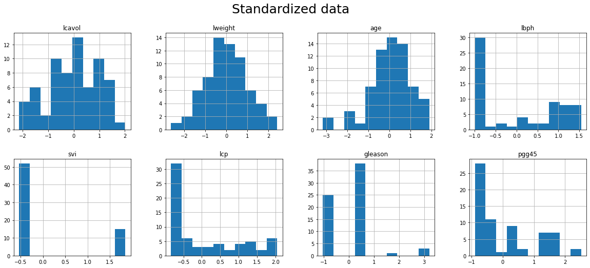
26. Show the histogram of each variables of predictorsTrain_std in a single figure
- Use argument figsize to enlarge the figure if needed
- Hint: which kind of difference can you see in the histograms?
print("Now all the variables are centered at 0 and they variance equal to 1. So we can compare them in a better way.")
fig = plt.figure()

predictorsTrain_std.hist(grid=True, figsize=(20,8), layout = (2,4))

plt.suptitle("Standardized data", fontsize=25)
fig.tight_layout()

plt.show()
Now all the variables are centered at 0 and they variance equal to 1. So we can compare them in a better way.


<Figure size 432x288 with 0 Axes>
Linear Regression #
27. Generate a linear regression model using `predictorsTrain_std` as dependent variables and `lpsaTrain` as independent variable
Hint: find a function for linear regression model learning in sklearn (fit)
How do you set parameter fit_intercept? Why?
The parameter
fit_interceptspecifies whether to calculate the intercept for this model:- If False, then the y-intercept to 0 (it is forced to 0);
- if True, then the y-intercept will be determined by the line of best fit (it’s allowed to “fit” the y-axis).
As default
fit_interceptis True and it is good for us.How do you set parameter normalize? Why? Can this parameter be used to simplify the generation of the predictor matrix?
If
fit_intercept= False, then the parameternormalizeis ignored. Ifnormalize= True, the regressors X will be normalized before regression by subtracting the mean and dividing by the l2-norm.By default
normalize= False.We have already standardized our variables, so we set it as False.
# Create X_test
#predictorsTestMean = predictorsTest.mean()
predictorsTestStds = predictorsTest.std()
#predictorsTest_std = (predictorsTest - predictorsTestMeans)/predictorsTestStds # standardized cariables of predictorTrain
predictorsTest_std = (predictorsTest - predictorsTrainMeans)/predictorsTrainStds # standardized cariables of predictorTrain (BETTER WAY TO DO IT)
# Prepare the independent and dependent variables for the model

# Independent variables
X_train = predictorsTrain_std
X_test = predictorsTest_std

# Dependent variable
y_train = lpsaTrain
y_test = lpsaTest
linreg = LinearRegression() # we don't need to specify args, because the default ones are already good for us
linreg.fit(X_train,y_train)

# by default: fit_intercept = True and normalize = False
# This setting is good because we want to compute the intercept and we don't need to normalize X because we have already done it
LinearRegression()
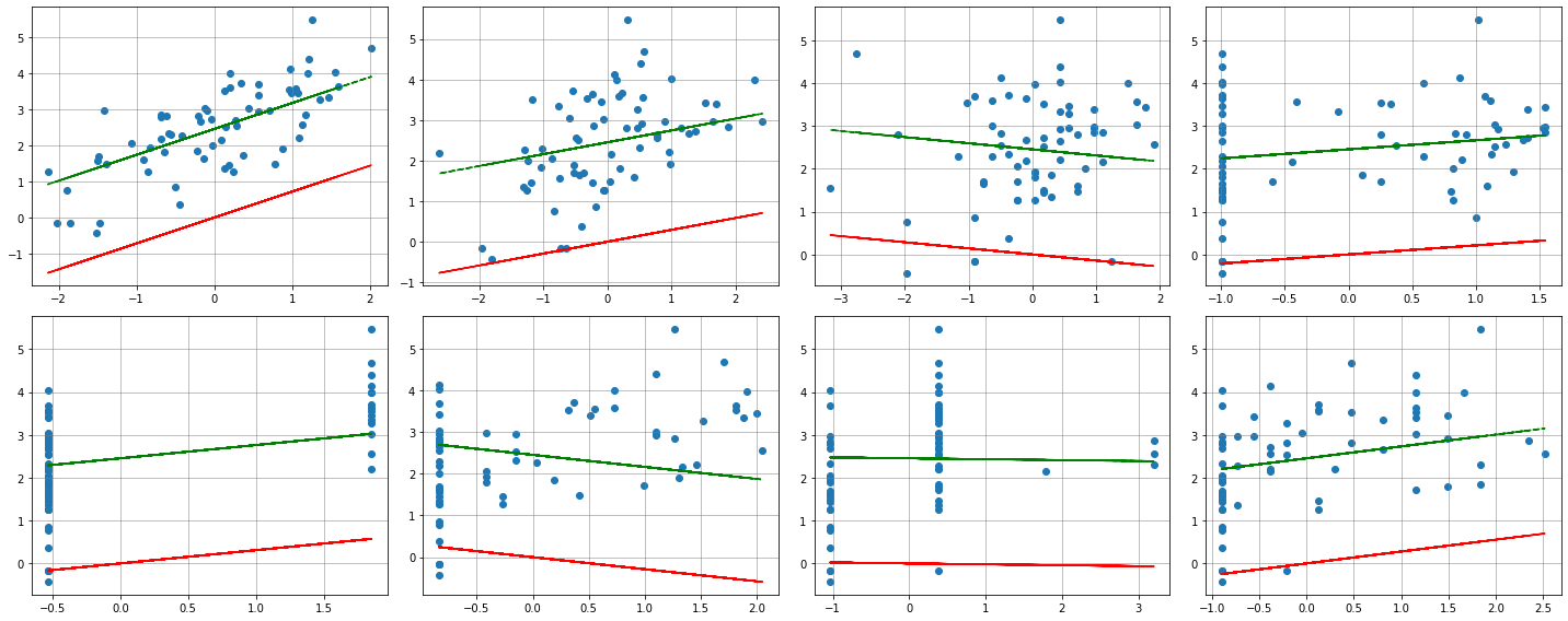
Difference in setting up fit_intercept in LinearRegression() #
# Difference in setting up fit_intercept

lr_fi_true = LinearRegression(fit_intercept=True)
lr_fi_false = LinearRegression(fit_intercept=False)

lr_fi_true.fit(X_train, y_train)
lr_fi_false.fit(X_train, y_train)

print('Intercept when fit_intercept=True : {:.5f}'.format(lr_fi_true.intercept_))
print('Intercept when fit_intercept=False : {:.5f}'.format(lr_fi_false.intercept_))

# FIGURE
# SOURCE: https://stackoverflow.com/questions/46779605/in-the-linearregression-method-in-sklearn-what-exactly-is-the-fit-intercept-par

# fig properties
row = 2
col = 4
width = 20
height = 8

# initialize the figure
fig, axes = plt.subplots(row, col,figsize=(width,height))

for ax,variable in zip(axes.flatten(),X_train.columns.tolist()):
    ax.scatter(X_train[variable],y_train, label='Actual points')

    ax.grid(color='grey', linestyle='-', linewidth=0.5)

    idx = X_train.columns.get_loc(variable) # get corresponding column index to access the right coeff

    lr_fi_true_yhat = np.dot(X_train[variable], lr_fi_true.coef_[idx]) + lr_fi_true.intercept_
    lr_fi_false_yhat = np.dot(X_train[variable], lr_fi_false.coef_[idx]) + lr_fi_false.intercept_

    ax.plot(X_train[variable], lr_fi_true_yhat, 'g--', label='fit_intercept=True')
    ax.plot(X_train[variable], lr_fi_false_yhat, 'r-', label='fit_intercept=False')

fig.tight_layout()

plt.show(fig) # force to show the plot after the print
Intercept when fit_intercept=True : 2.45235
Intercept when fit_intercept=False : 0.00000
lr_fi_true = LinearRegression(fit_intercept=True)
lr_fi_true.fit(X_train, y_train)
print(lr_fi_true.coef_,"\n",lr_fi_true.intercept_,"\n\n")

lr_fi_false = LinearRegression(fit_intercept=False)
lr_fi_false.fit(X_train, y_train)
print(lr_fi_true.coef_,"\n",lr_fi_false.intercept_)
[ 0.71640701  0.2926424  -0.14254963  0.2120076   0.30961953 -0.28900562
 -0.02091352  0.27734595]
 2.4523450850746262


[ 0.71640701  0.2926424  -0.14254963  0.2120076   0.30961953 -0.28900562
 -0.02091352  0.27734595]
 0.0
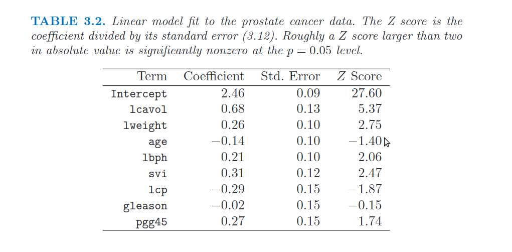
28. Show the parameters of the linear regression model computed above. Compare the parameters with those shown in Table 3.2 of the book (page 50)
col = ['Term','Coefficient'] # headers

intercept_val = np.array([linreg.intercept_]).round(2)
coeff_val = linreg.coef_.round(2)
intercept_label = np.array(['Intercept'])
coeff_label = X_train.columns.tolist()

terms = np.concatenate((intercept_val,coeff_val), axis=0)
coeffs = np.concatenate((intercept_label,coeff_label),axis=0)

table = np.column_stack((coeffs,terms))

print(tabulate(table, headers=col, tablefmt='fancy_grid'))
╒═══════════╤═══════════════╕
│ Term      │   Coefficient │
╞═══════════╪═══════════════╡
│ Intercept │          2.45 │
├───────────┼───────────────┤
│ lcavol    │          0.72 │
├───────────┼───────────────┤
│ lweight   │          0.29 │
├───────────┼───────────────┤
│ age       │         -0.14 │
├───────────┼───────────────┤
│ lbph      │          0.21 │
├───────────┼───────────────┤
│ svi       │          0.31 │
├───────────┼───────────────┤
│ lcp       │         -0.29 │
├───────────┼───────────────┤
│ gleason   │         -0.02 │
├───────────┼───────────────┤
│ pgg45     │          0.28 │
╘═══════════╧═══════════════╛
# We can compare the above correlation matrix with the one in the book:
Image("../input/prostate-data/tab2.png")

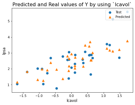
29. Compute the coefficient of determination of the prediction
For coefficient of determination we mean \(R^{2}\).
y_predicted = linreg.predict(X_test)
y_predicted
array([1.96903844, 1.16995577, 1.26117929, 1.88375914, 2.54431886,
       1.93275402, 2.04233571, 1.83091625, 1.99115929, 1.32347076,
       2.93843111, 2.20314404, 2.166421  , 2.79456237, 2.67466879,
       2.18057291, 2.40211068, 3.02351576, 3.21122283, 1.38441459,
       3.41751878, 3.70741749, 2.54118337, 2.72969658, 2.64055575,
       3.48060024, 3.17136269, 3.2923494 , 3.11889686, 3.76383999])
score = r2_score(y_test,y_predicted) # goodness of fit measure for linreg
score2 = mean_squared_error(y_test,y_predicted)

print(f"The coefficient of determination (i.e. R^2) of the prediction is {round(score,3)}\n\
The mean squared error is: {round(score2,3)}.\n\
The root of the mean squared error is {round(np.sqrt(score2),3)}")
The coefficient of determination (i.e. R^2) of the prediction is 0.503
The mean squared error is: 0.521.
The root of the mean squared error is 0.722
plt.figure(figsize=[7,5])
plt.scatter(X_test['lcavol'],y_test, marker='o', s = 50)
plt.scatter(X_test['lcavol'],y_predicted, marker='^', s = 50)
plt.title('Predicted and Real values of Y by using `lcavol`',fontsize=16)

plt.legend(labels = ['Test','Predicted'],loc = 'upper right')
plt.xlabel('lcavol',fontsize=12)
plt.ylabel('lpsa',fontsize=12)

plt.show()
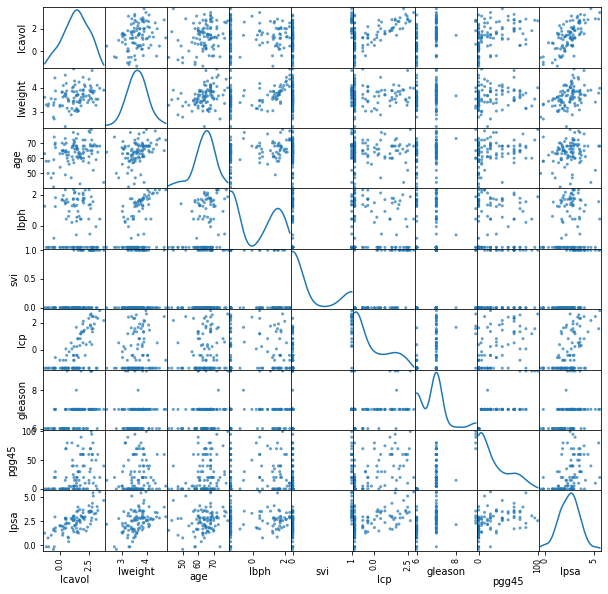
data_all = pd.read_csv('../input/prostate-data/prostate.data',sep='\t')
data_all = data_all.drop(labels = ['Unnamed: 0'],axis=1)
featuresToPlot = data_all.columns.tolist()
dataToPlot = data_all[featuresToPlot]

pd.plotting.scatter_matrix(dataToPlot, alpha = 0.7, diagonal = 'kde', figsize=(10,10))

plt.show()
plt.figure(figsize=[7,5])
plt.scatter(predictorsTrain_std['lweight'],lpsaTrain, marker='o', s = 50)
plt.title('Linear relationship btw `lweight` and  `lpsa`',fontsize=16)

plt.xlabel('lweight',fontsize=12)
plt.ylabel('lpsa',fontsize=12)

plt.show()

# in this case linear regression is nice!
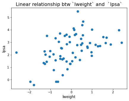
We can see how these relationships are linear. We can see linearity from the plot.
r2test = round(linreg.score(X_test,lpsaTest),2)
r2train = round(linreg.score(X_train,lpsaTrain),2)

print(f"Coefficient of determination for Test set is {r2test}\n\
Coefficient of determination for Test set is {r2train}") # it's higher because the model is created by using train set
Coefficient of determination for Test set is 0.5
Coefficient of determination for Test set is 0.69
30. Compute the standard errors, the Z scores (Student’s t statistics) and the related p-values
- Hint: use library `statsmodels instead of sklearn
- Hint: compare the results with those in Table 3.2 of the book (page 50)
y_predicted = linreg.predict(X_test)

X_trainC = sm.add_constant(X_train) # We need this in order to have an intercept
                        # otherwise we will no have the costant (it would be 0)

model = sm.OLS(y_train,X_trainC) # define the OLS (Ordinary Least Square - Linear Regression model)

results = model.fit() # fit the model

results.params # Coefficients of the model
results.summary(slim=True)

# Adjusted R^2 is the r^2 scaled by the number of parameters in the model
# F-statistics tells if the value of R^2 is significant or not.
| Dep. Variable: | lpsa | R-squared: | 0.694 |
|---|---|---|---|
| Model: | OLS | Adj. R-squared: | 0.652 |
| No. Observations: | 67 | F-statistic: | 16.47 |
| Covariance Type: | nonrobust | Prob (F-statistic): | 2.04e-12 |
| coef | std err | t | P>|t| | [0.025 | 0.975] | |
|---|---|---|---|---|---|---|
| const | 2.4523 | 0.087 | 28.182 | 0.000 | 2.278 | 2.627 |
| lcavol | 0.7164 | 0.134 | 5.366 | 0.000 | 0.449 | 0.984 |
| lweight | 0.2926 | 0.106 | 2.751 | 0.008 | 0.080 | 0.506 |
| age | -0.1425 | 0.102 | -1.396 | 0.168 | -0.347 | 0.062 |
| lbph | 0.2120 | 0.103 | 2.056 | 0.044 | 0.006 | 0.418 |
| svi | 0.3096 | 0.125 | 2.469 | 0.017 | 0.059 | 0.561 |
| lcp | -0.2890 | 0.155 | -1.867 | 0.067 | -0.599 | 0.021 |
| gleason | -0.0209 | 0.143 | -0.147 | 0.884 | -0.306 | 0.264 |
| pgg45 | 0.2773 | 0.160 | 1.738 | 0.088 | -0.042 | 0.597 |
Notes:
[1] Standard Errors assume that the covariance matrix of the errors is correctly specified.
# We can compare the above correlation matrix with the one in the book:
Image("../input/prostate-data/tab2.png")