- Welcome to Congo! :tada:/
- Posts/
- Some exercise about Statistical Learning/
- SL4: Analysis of Prostate Cancer dataset – shrinkage methods/
SL4: Analysis of Prostate Cancer dataset – shrinkage methods
17 mins
Table of Contents
# data analysis and wrangling
import numpy as np # linear algebra
import pandas as pd # data processing, CSV file I/O (e.g. pd.read_csv)
# import random as rnd

# visualization
import seaborn as sns
import matplotlib.pyplot as plt
# %matplotlib inline

# machine learning
from sklearn.linear_model import LinearRegression
from sklearn.linear_model import Ridge
from sklearn.linear_model import RidgeCV
from sklearn.linear_model import Lasso
from sklearn.linear_model import lasso_path
from sklearn.linear_model import LassoCV
from sklearn.metrics import r2_score
from sklearn.metrics import mean_squared_error

import statsmodels.api as sm

from IPython.display import Image # to visualize images
from tabulate import tabulate # to create tables

import os
for dirname, _, filenames in os.walk('/kaggle/input'):
    for filename in filenames:
        print(os.path.join(dirname, filename))
/kaggle/input/prostate-data/tab4.png
/kaggle/input/prostate-data/tab4-no-cap.png
/kaggle/input/prostate-data/tab3.png
/kaggle/input/prostate-data/prostate.data
/kaggle/input/prostate-data/tab.png
/kaggle/input/prostate-data/tab2.png
1. Open your kernel SL_EX2_ProstateCancer_Surname in Kaggle
2. Generate a copy called SL_EX4_Prostate_Shrinkage_Surname by the Fork button
3. Import Ridge from sklearn.linear_model
Data acquisition #
# Load the Prostate Cancer dataset
data = pd.read_csv('../input/prostate-data/prostate.data',sep='\t')
# Save "train" and lpsa" columns into Pandas Series variables
train = data['train']
lpsa = data['lpsa']

# Drop "train" and lpsa" variable from data
data = data.drop(columns=['Unnamed: 0','lpsa','train'],axis=1)
Data pre-processing #
## X VARIABLE:
# Split the data in train and test sets
dataTrain = data.loc[train == 'T'] # Obviously, len(idx)==len(dataTrain) is True!
dataTest = data.loc[train == 'F']

# Rename these two variables as "predictorsTrain" and "predictorsTest"
predictorsTrain = dataTrain
predictorsTest = dataTest


## Y VARIABLE:
# Split the "lpsa" in train and test sets
lpsaTrain = lpsa.loc[train == 'T']
lpsaTest = lpsa.loc[train == 'F']
Standardization #
# Standardize "predictorsTrain"
predictorsTrainMeans = predictorsTrain.mean()
predictorsTrainStds = predictorsTrain.std()
predictorsTrain_std = (predictorsTrain - predictorsTrainMeans)/predictorsTrainStds # standardized variables of predictorTrain

# Standardize "predictorsTest" (using the mean and std of predictorsTrain, it's better!)
predictorsTest_std = (predictorsTest - predictorsTrainMeans)/predictorsTrainStds # standardized variables of predictorTest

# Standardize all the data together (necessary for CV)
predictors = data
predictors_std = (predictors - predictors.mean())/predictors.std()
Split into Training and Test sets #
## TRAINING SET
X_train = predictorsTrain_std
Y_train = lpsaTrain

## TEST SET
X_test = predictorsTest_std
Y_test = lpsaTest

## All the data standardized
X = predictors_std
Y = lpsa
Ridge regression #
4. Starting from standardized data, generate a ridge regression model with \(\alpha\)=1.0 (called \(\lambda\) in the slides)
## Ridge Regression model trained on training set
ridge = Ridge(alpha=1, fit_intercept=True)
ridge.fit(X_train,Y_train); # if alpha=0, then Ridge coincides with OLS
5. Show model’s coefficients, intercept and score (on both the training and the test set)
## For Ridge model

# Stats on train
R2_train_ridge = ridge.score(X_train,Y_train)

# Stats on test
R2_test_ridge = ridge.score(X_test,Y_test)

round_coef = 3
print(f"\
About the the Ridge regression model for alpha = 1:\n\
* intercept: {ridge.intercept_.round(round_coef)}\n\
* model coefficients:: {ridge.coef_.round(round_coef).tolist()}\n\
* R^2 on training set: {R2_train_ridge.round(round_coef)}\n\
* R^2 on test set: {R2_test_ridge.round(round_coef)}\n\
")
About the the Ridge regression model for alpha = 1:
* intercept: 2.452
* model coefficients:: [0.69, 0.292, -0.135, 0.21, 0.304, -0.256, -0.011, 0.258]
* R^2 on training set: 0.694
* R^2 on test set: 0.512
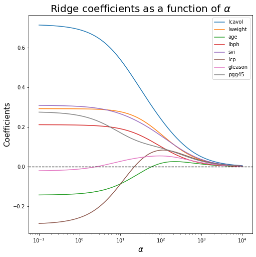
6. Plot Ridge coefficients as functions of the regularization parameter alpha
# create a vector of alphas
alphas = np.logspace(start = -1, stop = 4, num = 200, base = 10) # regularization params [base**start,base**end]

coefs_r = [] # lists to store model coeffs

for a in alphas:

    # Compute the Ridge model
    reg = Ridge(alpha=a, fit_intercept=True)
    reg.fit(X_train,Y_train)

    # Store coefficient
    coefs_r.append(reg.coef_)
# fig
width, height = 8, 8
fig, ax = plt.subplots(figsize=(width,height))

ax.plot(alphas, coefs_r)
ax.axhline(0, linestyle="--", linewidth=1.25, color="black")  # horizontal line

ax.set_xscale('log')
# ax.set_xlim(ax.get_xlim()[::-1]) # reverse the x-axis

ax.set_xlabel(r"$\alpha $", fontsize=15)
ax.set_ylabel("Coefficients", fontsize=15)
ax.set_title(r"Ridge coefficients as a function of $\alpha$", fontsize=20)
ax.legend(X_train.columns.tolist())

plt.show()
Ridge coefficients as functions of the effective DoF #
The effective degree of freedom of the Ridge regression is \[\text{df} (\alpha ) = \sum_{i=1}^{n} \dfrac{d_i^2}{d_i^2+\alpha}\] where \(d_i\) are singular values of \(X\).
In a linear-regression fit with p variables, the degrees-of-freedom of the fit is \(df(\alpha)=p\), the number of free parameters.
The idea is that although all p coefficients in a ridge fit will be non-zero, they are fit in a restricted fashion controlled by \(\alpha\). Note that when we have no regularization \(df(0)=p\) .
# Compute effective DoF

df_r = []
s2 = np.linalg.svd(X_train, compute_uv=False)**2   # singular values squared

for a in alphas:
    tmp = s2/(s2+a)
    df_r.append(tmp.sum())
# fig
width, height = 8, 8
palette = 'darkblue'
fig, ax = plt.subplots(figsize=(width,height))

ax.plot(df_r, coefs_r, color=palette)
#ax.axvline(5, linestyle=":", linewidth=1.25, color="red")     # vertical line
ax.axhline(0, linestyle="--", linewidth=1.25, color="black")  # horizontal line

ax.set_xlabel(r"df($\alpha $)", fontsize=15)
ax.set_ylabel("Coefficients", fontsize=15)
ax.set_title("Ridge coefficients as functions of the effective DoF", fontsize=20)
ax.set_xlim(-0.5, 9)

# Annotate the name of each variable at the last value
coords = zip([8]*len(coefs_r[0]),coefs_r[0]) # last value where I want to annotate the corresponding label
labels = X_train.columns.tolist()

for coord,lab in zip(coords,labels):
    ax.annotate(xy=coord,                    # The point (x, y) to annotate.
                xytext=coord,                # The position (x, y) to place the text at.
                textcoords='offset points',
                text=lab,
                verticalalignment='center')

plt.show()
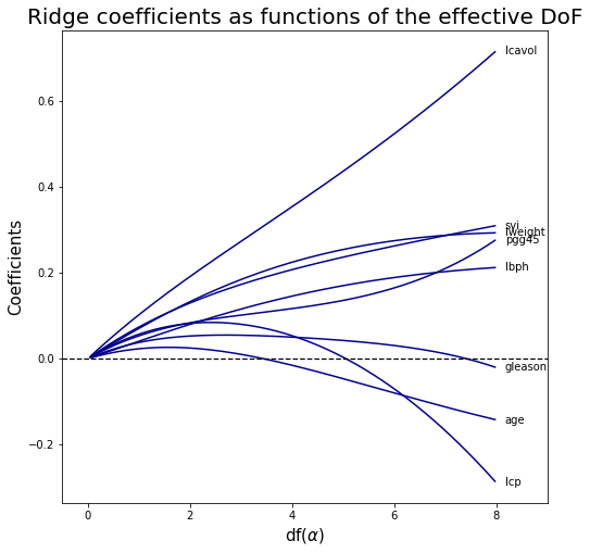
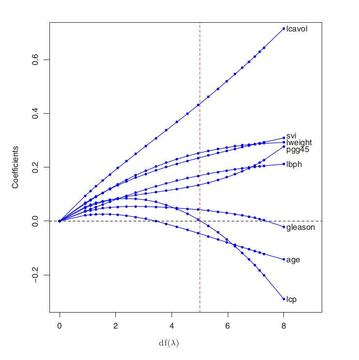
# We can compare the above chart with the one in the book (figure 3.8):
scale = 70
Image("../input/prostate-data/tab4-no-cap.png", width = width*scale, height = height*scale)
Ridge regression LOOCV #
7. Find the best regularization parameter by cross-validation using leave-one-out
- Use only the training set (97 observations).
- Use store_cv_values=True to get the leave-one-out errors.
- The cv_values_ in the result object provided by RidgeCV contains one row for each observation (97 rows) and one column for each alpha in alphas (100 columns).
Cell i,j contains the leave-one-out mean squared error on the i-th observation given the j-th alpha.
By computing the mean by column of cv_values_ you obtain the average cross-validation error for each alpha. This is the value that has to be minimized (see next step).
# Create and train the model using all the data
alphas = np.logspace(start=-1,stop=4,num=200,base=10.0)

# cv = None, to use the Leave-One-Out cross-validation
ridgeLOO = RidgeCV(alphas = alphas, cv=None, fit_intercept = True, store_cv_values = True)
ridgeLOO.fit(X,Y)

cvVal = ridgeLOO.cv_values_  # cvVal[i,j] = LOO MSE on the i-th observation given the j-th alpha
cvMeans = np.mean(cvVal,axis=0)
cvStd = np.std(cvVal,axis=0)

print("The shape is: ",np.shape(cvVal)) # contains one row for each observation and one column for each alpha in alphas
The shape is: (97, 200)
## Best regularization parameter: identify the minimum LOOCV MSE and the related alpha

min_val = min(cvMeans)
# min_val = abs(ridgeLOO.best_score_)   # alternative way
min_alpha = ridgeLOO.alpha_
# min_alpha = ridgeLOO.alphas[np.argmin(cvMeans)]   # alternative way

print(f"\
The best regularization parameter is \u03B1={min_alpha.round(3)}, with corresponding LOOCV MSE equal to {min_val.round(3)}.\
")
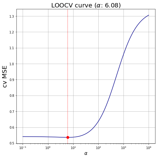
The best regularization parameter is α=6.08, with corresponding LOOCV MSE equal to 0.536.
9. Identify the minimum leave-one-out cross-validation error and the related alpha, model coefficients and performance
## Perform the Ridge regression on the best alpha
ridgeLOO_best = RidgeCV(alphas = min_alpha, fit_intercept = True)
ridgeLOO_best.fit(X,Y)

# Stats on train
R2_train_ridgeLOO_best = ridgeLOO_best.score(X_train,Y_train)

# Stats on test
R2_test_ridgeLOO_best = ridgeLOO_best.score(X_test,Y_test)

# print some info about Ridge CV
round_coef = 3

print(f"\
For this value of \u03B1={min_alpha.round(round_coef)} we have the following parameters:\n\
* intercept: {ridgeLOO_best.intercept_.round(round_coef)}\n\
* model coefficients: {ridgeLOO_best.coef_.round(round_coef).tolist()}\n\
* R^2 on training set: {R2_train_ridgeLOO_best.round(round_coef)}\n\
* R^2 on test set: {R2_test_ridgeLOO_best.round(round_coef)}\n\
")
For this value of α=6.08 we have the following parameters:
* intercept: 2.478
* model coefficients: [0.59, 0.26, -0.128, 0.126, 0.287, -0.065, 0.045, 0.099]
* R^2 on training set: 0.67
* R^2 on test set: 0.609
8. Plot the leave-one-out cross-validation curve
- Hint: plot the alphas vector against the average cross-validation error for each alpha computed at the last point
# fig
width, height = 8, 8
palette = 'darkblue'
fig, ax = plt.subplots(figsize=(width,height))

# straight lines
ax.plot(ridgeLOO.alphas, cvMeans, color='darkblue')

ax.plot(min_alpha, min_val, marker= 'o', markersize = 8, color='r')
ax.axvline(min_alpha, linestyle=":", linewidth=1.5, color="red") # vertical line

ax.set_xlabel(r"$\alpha$", fontsize=15)
ax.set_ylabel("cv MSE", fontsize=20)
ax.set_title(fr"LOOCV curve ($\alpha$: {ridgeLOO.alpha_.round(3)})", fontsize=20)
ax.set_xscale('log')
ax.grid(color='grey', linestyle='-', linewidth=0.5);
# ax.set_xlim(ax.get_xlim()[::-1]) # reverse the x-axis

plt.show()
Ridge regression with 10-Folds Cross Validation #
10. Identify the minimum 10-folds cross-validation error and the related alpha, model coefficients and performance
# store_cv_values = False otherwise it is incompatible with cv!=none
ridge_10cv = RidgeCV(alphas = alphas, fit_intercept = True, store_cv_values = False, cv = 10);
ridge_10cv.fit(X,Y);
# Best regularization parameter: identify the minimum LOO CV error and the related alpha
min_alpha_10cv = ridge_10cv.alpha_
min_val_10cv = abs(ridge_10cv.best_score_) # loocv of 10cv

print(f"\
The best regularization parameters is \u03B1={min_alpha_10cv.round(3)}, with corresponding Leave-One-Out MSE equal to: {min_val_10cv.round(3)}\n\
")
The best regularization parameters is α=207.292, with corresponding Leave-One-Out MSE equal to: 52.447
## Perform the Ridge regression with 10 folds on the best alpha (in order to perform on train and test sets)
ridge_10cv_best = RidgeCV(alphas = min_alpha_10cv, fit_intercept = True)
ridge_10cv_best.fit(X,Y)

# Stats on train
R2_train_ridge_10cv_best = ridge_10cv_best.score(X_train,Y_train)

# Stats on test
R2_test_ridge_10cv_best = ridge_10cv_best.score(X_test,Y_test)

# print some info about Ridge CV
round_coef = 3

print(f"\
For this value of \u03B1={min_alpha_10cv.round(round_coef)} we have the following parameters:\n\
* intercept: {ridge_10cv_best.intercept_.round(round_coef)}\n\
* model coefficients: {ridge_10cv_best.coef_.round(round_coef).tolist()}\n\
* R^2 on training set: {R2_train_ridge_10cv_best.round(round_coef)}\n\
* R^2 on test set: {R2_test_ridge_10cv_best.round(round_coef)}\n\
")
For this value of α=207.292 we have the following parameters:
* intercept: 2.478
* model coefficients: [0.195, 0.118, 0.01, 0.047, 0.131, 0.101, 0.058, 0.068]
* R^2 on training set: 0.468
* R^2 on test set: 0.459
Comparison between Ridge LOO CV and Ridge 10 Folds CV #
# table
round_coef = 3
headers = ['Term','Ridge LOOCV', 'Ridge 10-CV']

# labels (0-th column)
intercept_label = np.array(['Intercept'])
alpha_label = np.array(['Best Alpha'])
coefs_label = X_train.columns.tolist()
labels = np.concatenate((intercept_label,alpha_label,coefs_label),axis=0)

# ridge LOOCV column values
model = ridgeLOO_best
model_intercept_val = np.array([model.intercept_])
model_alpha_val = np.array([model.alpha_])
model_coefs_val = model.coef_
ridgeLOO_values = np.concatenate((model_intercept_val,model_alpha_val,model_coefs_val), axis=0).round(round_coef)

# ridge 10CV column values
model = ridge_10cv_best
model_intercept_val = np.array([model.intercept_])
model_alpha_val = np.array([model.alpha_])
model_coefs_val = model.coef_
ridge_10cv_values = np.concatenate((model_intercept_val,model_alpha_val,model_coefs_val), axis=0).round(round_coef)

table = np.column_stack((labels, ridgeLOO_values, ridge_10cv_values))

print(tabulate(table, headers=headers, tablefmt='fancy_grid'))
╒════════════╤═══════════════╤═══════════════╕
│ Term       │   Ridge LOOCV │   Ridge 10-CV │
╞════════════╪═══════════════╪═══════════════╡
│ Intercept  │         2.478 │         2.478 │
├────────────┼───────────────┼───────────────┤
│ Best Alpha │         6.08  │       207.292 │
├────────────┼───────────────┼───────────────┤
│ lcavol     │         0.59  │         0.195 │
├────────────┼───────────────┼───────────────┤
│ lweight    │         0.26  │         0.118 │
├────────────┼───────────────┼───────────────┤
│ age        │        -0.128 │         0.01  │
├────────────┼───────────────┼───────────────┤
│ lbph       │         0.126 │         0.047 │
├────────────┼───────────────┼───────────────┤
│ svi        │         0.287 │         0.131 │
├────────────┼───────────────┼───────────────┤
│ lcp        │        -0.065 │         0.101 │
├────────────┼───────────────┼───────────────┤
│ gleason    │         0.045 │         0.058 │
├────────────┼───────────────┼───────────────┤
│ pgg45      │         0.099 │         0.068 │
╘════════════╧═══════════════╧═══════════════╛
Lasso regression #
11. Import Lasso from sklearn.linear_model
✅
12. Generate a lasso regression model with a specific regularization parameter alpha=0.1
# Create a Lasso regression model
lasso = Lasso(alpha = 0.1)
lasso.fit(X_train,Y_train);
14 Show model’s coefficients, intercept and score (on both the training and the test set)
# Stats on train
R2_train_lasso = lasso.score(X_train,Y_train)

# Stats on test
R2_test_lasso = lasso.score(X_test,Y_test)

round_coef = 3

print(f"\
About the the Lasso regression model:\n\
* intercept: {lasso.intercept_.round(round_coef)}\n\
* model coefficients: {lasso.coef_.round(round_coef).tolist()}\n\
* R^2 on training set: {R2_train_lasso.round(round_coef)}\n\
* R^2 on test set: {R2_test_lasso.round(round_coef)}\n\
")
About the the Lasso regression model:
* intercept: 2.452
* model coefficients: [0.575, 0.23, -0.0, 0.105, 0.172, 0.0, 0.0, 0.065]
* R^2 on training set: 0.648
* R^2 on test set: 0.569
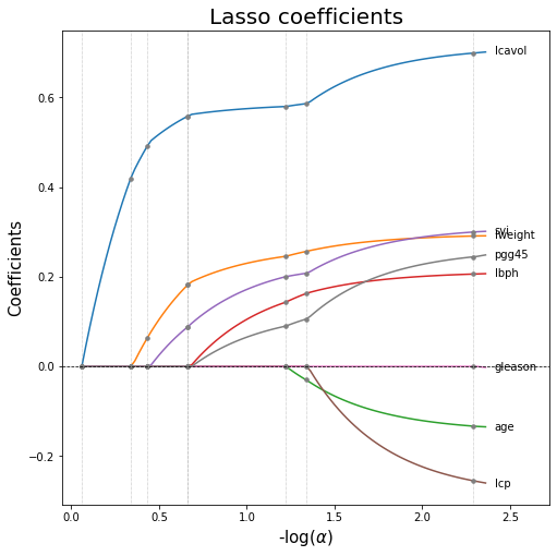
15. Plot Lasso coefficients as a function of the regularization parameter
# Lasso path: coefficients as functions of the regularization parameters

# we can set either alphas or eps: the smaller eps, the longer the path is
alphas_lasso, coefs_lasso, _ = lasso_path(X_train, Y_train, eps = 5e-3)
# For each coefficient I compute the first index in which it becomes zero.
nz_list = list((coefs_lasso !=0).argmax(axis=1)-1)
# fig
width, height = 8, 8
fig, ax = plt.subplots(figsize=(width,height))

xx = -np.log10(alphas_lasso) # neg_log_alphas_lasso

for coef in coefs_lasso:
    ax.plot(xx, coef)

# Info about when coefs are shrunken to 0
for nz in nz_list:
    ax.axvline(xx[nz], linestyle=":", linewidth=0.5, color="grey") # vertical line

    # dots where coefs become zero
    for coef in coefs_lasso:
        ax.plot(xx[nz], coef[nz],  linestyle='None', marker = 'o', markersize=3.5, color = 'grey')

ax.axhline(y=0, linestyle='--',linewidth=0.75, color='black') # horizontal line
#ax.grid(color='grey', linestyle='-', linewidth=0.5);
ax.set_xlabel(r"-log($\alpha$)", fontsize=15)
ax.set_ylabel("Coefficients", fontsize=15)
ax.set_title("Lasso coefficients", fontsize=20)


## Annotate the name of each variable at the last value

ax.set_xlim(-0.05, ax.get_xlim()[1]*1.1)      # enlarge xaxis
alpha_end = xx[-1]*1.015                      # last value of alpha
last_val = [last for *_, last in coefs_lasso] # last value of all the 8 coeffs

coords = zip([alpha_end]*8,last_val)
labels = X_train.columns.tolist()

for coord,lab in zip(coords,labels):
    ax.annotate(xy=coord,            # The point (x, y) to annotate.
                xytext=coord,        # The position (x, y) to place the text at.
                textcoords='offset points',
                text=lab,
                verticalalignment='center')

plt.show()
16. Find the best regularization parameter by cross-validation
- Hint: use function LassoCV from sklearn
- Test different number of cv folds
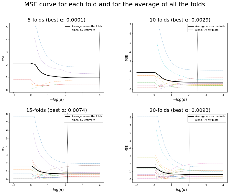
17. Plot the mean square error curve for each fold and for the average of all the folds
## Some params
cvFolds = np.arange(start = 5, stop = 25, step  = 5)
alpha_lasso_cv = np.logspace(-4,1,100,10)

# where we store some info
best_alpha, performances_lasso_cv = [], []
intercepts_lasso_cv, model_coefs = [], []
# Initialize the fig
nrow, ncol = 2, 2
width, height = 16, 12 # single subplot
fig, axes = plt.subplots(nrow,ncol,figsize=(width,height))

for folds, ax in zip(cvFolds,axes.flatten()):

    lasso_cv = LassoCV(cv=folds, alphas=alpha_lasso_cv)
    lasso_cv.fit(X_train,Y_train) # fitting the model using n-folds

    # R^2 train
    pred_train_lasso_cv = lasso_cv.predict(X_train)
    Rsquared_train_lasso_cv = lasso_cv.score(X_train,Y_train)
    # R^2 test
    pred_test_lasso_cv = lasso_cv.predict(X_test)
    Rsquared_test_lasso_cv = lasso_cv.score(X_test,Y_test)

    #store some info
    best_alpha.append(lasso_cv.alpha_)
    model_coefs.append(lasso_cv.coef_)
    intercepts_lasso_cv.append(lasso_cv.intercept_)
    performances_lasso_cv.append([Rsquared_train_lasso_cv,Rsquared_test_lasso_cv])

    m_log_alphas = -np.log10(lasso_cv.alphas_)
    ax.plot(m_log_alphas, lasso_cv.mse_path_, linestyle="--", linewidth=0.5)
    ax.plot(m_log_alphas, lasso_cv.mse_path_.mean(axis=1), color="black", label="Average across the folds", linewidth=2.5)

    ax.axvline(-np.log10(lasso_cv.alpha_), linestyle=":", color="black", label="alpha: CV estimate") # best alpha

    #ax.grid(color='grey', linestyle='-', linewidth=0.5);
    ax.set_xlabel(r"$-log(\alpha)$", fontsize=15)
    ax.set_ylabel("MSE", fontsize=12)
    ax.set_title(f"{folds}-folds (best \u03B1: {lasso_cv.alpha_.round(4)})", fontsize=20)
    ax.legend(loc='upper right')


plt.axis("tight")

# set the spacing between subplots
plt.subplots_adjust(wspace=0.3, hspace=0.3)
plt.suptitle("MSE curve for each fold and for the average of all the folds",fontsize=25)
plt.show()
# Best regularization parameter by cross-validation
print("Best regularization parameter \u03B1:")
for nfolds, alpha in zip(cvFolds,best_alpha):
    print(f" * For {nfolds}-folds: {alpha.round(4)}")
Best regularization parameter α:
 * For 5-folds: 0.0001
 * For 10-folds: 0.0029
 * For 15-folds: 0.0074
 * For 20-folds: 0.0093
18. Show the best alpha, model coefficients and performance on training and test set
## For Lasso_cv model

round_coef = 3
print("Some stats about the performance of Lasso CV with different folds:\n")
for k in range(0,len(cvFolds)):
    print(f"* For {cvFolds[k]}-folds:\n\
    - best \u03B1: {best_alpha[k].round(round_coef)}\n\
    - intercept: {intercepts_lasso_cv[k].round(round_coef)}\n\
    - coefficients: {model_coefs[k].round(round_coef).tolist()}\n\
    - score on training set: {performances_lasso_cv[k][0].round(round_coef)}\n\
    - score on test set: {performances_lasso_cv[k][1].round(round_coef)}\n\
    ")
Some stats about the performance of Lasso CV with different folds:

* For 5-folds:
    - best α: 0.0
    - intercept: 2.452
    - coefficients: [0.716, 0.293, -0.142, 0.212, 0.309, -0.288, -0.02, 0.277]
    - score on training set: 0.694
    - score on test set: 0.504

* For 10-folds:
    - best α: 0.003
    - intercept: 2.452
    - coefficients: [0.706, 0.292, -0.137, 0.209, 0.304, -0.27, -0.008, 0.258]
    - score on training set: 0.694
    - score on test set: 0.511

* For 15-folds:
    - best α: 0.007
    - intercept: 2.452
    - coefficients: [0.692, 0.289, -0.127, 0.204, 0.295, -0.241, -0.0, 0.237]
    - score on training set: 0.694
    - score on test set: 0.521

* For 20-folds:
    - best α: 0.009
    - intercept: 2.452
    - coefficients: [0.687, 0.287, -0.123, 0.202, 0.29, -0.228, -0.0, 0.23]
    - score on training set: 0.693
    - score on test set: 0.524
Comparison between Lasso with different CV folds #
# table
round_coef = 3
headers = ['Term','Lasso CV\n(5-folds)', 'Lasso CV\n(10-folds)', 'Lasso CV\n(15-folds)', 'Lasso CV\n(20-folds)']

lasso_cv_values = []

# labels (0-th column)
intercept_label = np.array(['Intercept'])
alpha_label = np.array(['Best Alpha'])
coefs_label = X_train.columns.tolist()
labels = np.concatenate((intercept_label,alpha_label,coefs_label),axis=0)


for idx in range(0,4):
    model_intercept_val = np.array([intercepts_lasso_cv[idx]])
    model_alpha_val = np.array([best_alpha[idx]])
    model_coefs_val = model_coefs[idx]

    tmp = np.concatenate((model_intercept_val,model_alpha_val,model_coefs_val), axis=0).round(round_coef)

    lasso_cv_values.append(tmp)

# table = np.column_stack((labels,lasso_cv_values))
table = np.column_stack((labels, lasso_cv_values[0], lasso_cv_values[1], lasso_cv_values[2], lasso_cv_values[3]))


print(tabulate(table, headers=headers, tablefmt='fancy_grid'))
╒════════════╤═════════════╤══════════════╤══════════════╤══════════════╕
│ Term       │    Lasso CV │     Lasso CV │     Lasso CV │     Lasso CV │
│            │   (5-folds) │   (10-folds) │   (15-folds) │   (20-folds) │
╞════════════╪═════════════╪══════════════╪══════════════╪══════════════╡
│ Intercept  │       2.452 │        2.452 │        2.452 │        2.452 │
├────────────┼─────────────┼──────────────┼──────────────┼──────────────┤
│ Best Alpha │       0     │        0.003 │        0.007 │        0.009 │
├────────────┼─────────────┼──────────────┼──────────────┼──────────────┤
│ lcavol     │       0.716 │        0.706 │        0.692 │        0.687 │
├────────────┼─────────────┼──────────────┼──────────────┼──────────────┤
│ lweight    │       0.293 │        0.292 │        0.289 │        0.287 │
├────────────┼─────────────┼──────────────┼──────────────┼──────────────┤
│ age        │      -0.142 │       -0.137 │       -0.127 │       -0.123 │
├────────────┼─────────────┼──────────────┼──────────────┼──────────────┤
│ lbph       │       0.212 │        0.209 │        0.204 │        0.202 │
├────────────┼─────────────┼──────────────┼──────────────┼──────────────┤
│ svi        │       0.309 │        0.304 │        0.295 │        0.29  │
├────────────┼─────────────┼──────────────┼──────────────┼──────────────┤
│ lcp        │      -0.288 │       -0.27  │       -0.241 │       -0.228 │
├────────────┼─────────────┼──────────────┼──────────────┼──────────────┤
│ gleason    │      -0.02  │       -0.008 │       -0     │       -0     │
├────────────┼─────────────┼──────────────┼──────────────┼──────────────┤
│ pgg45      │       0.277 │        0.258 │        0.237 │        0.23  │
╘════════════╧═════════════╧══════════════╧══════════════╧══════════════╛
Results and comparisons #
OLS
## For OLS model

## Create an OLS model fitted on training set
ols = LinearRegression(fit_intercept=True);
ols.fit(X_train,Y_train);

# Stats on train
R2_train_ols = ols.score(X_train,Y_train)

# Stats on test
R2_test_ols = ols.score(X_test,Y_test)

round_coef = 3
print(f"About the the OLS regression model:\n\
* coefficients: {ols.coef_.round(round_coef).tolist()}\n\
* intercept: {ols.intercept_.round(round_coef).round(round_coef)}\n\
* R^2 on training set: {R2_train_ols.round(round_coef)}\n\
* R^2 on test set: {R2_test_ols.round(round_coef)}\n\
")
About the the OLS regression model:
* coefficients: [0.716, 0.293, -0.143, 0.212, 0.31, -0.289, -0.021, 0.277]
* intercept: 2.452
* R^2 on training set: 0.694
* R^2 on test set: 0.503
Best Subset Selection
## For Best Subset model - RSS - Andrea

predLabels = ['lcavol','svi','gleason']
X1, y1 = X_train[predLabels], Y_train
X2, y2 = X_test[predLabels], Y_test

# Create the linear model, fitting also the intecept (non-zero)
bssA = LinearRegression(fit_intercept = True).fit(X1,y1)

# Stats on train
R2_train_bssA = bssA.score(X1,y1)

# Stats on test
R2_test_bssA = bssA.score(X2,y2)

round_coef = 3
print(f"About the the Linear Regression regression model (choosing the predictors selected by BSS - performed by Andrea):\n\
* predictors: {predLabels}\n\
* coefficients: {bssA.coef_.round(round_coef).tolist()}\n\
* intercept: {bssA.intercept_.round(round_coef).round(round_coef)}\n\
* R^2 on training set: {R2_train_bssA.round(round_coef)}\n\
* R^2 on test set: {R2_test_bssA.round(round_coef)}\n\
")
About the the Linear Regression regression model (choosing the predictors selected by BSS - performed by Andrea):
* predictors: ['lcavol', 'svi', 'gleason']
* coefficients: [0.74, 0.225, 0.029]
* intercept: 2.452
* R^2 on training set: 0.561
* R^2 on test set: 0.635
Warning: Choosing the bestBest RSS for Best Selection, Backward Selection and Forward Selection gave the same choice of predictors: [lcavol, svi, gleason]
## For Best Subset model - RSS - Hastie and Tibshirani (book)

predLabels = ['lcavol','lweight']
X1, y1 = X_train[predLabels], Y_train
X2, y2 = X_test[predLabels], Y_test

# Create the linear model, fitting also the intecept (non-zero)
bssHT = LinearRegression(fit_intercept = True).fit(X1,y1)

# Stats on train
R2_train_bssHT = bssHT.score(X1,y1)

# Stats on test
R2_test_bssHT = bssHT.score(X2,y2)

round_coef = 3
print(f"About the the Linear Regression regression model (choosing the predictors selected by BSS - performed by HT):\n\
* predictors: {predLabels}\n\
* coefficients: {bssHT.coef_.round(round_coef).tolist()}\n\
* intercept: {bssHT.intercept_.round(round_coef).round(round_coef)}\n\
* R^2 on training set: {R2_train_bssHT.round(round_coef)}\n\
* R^2 on test set: {R2_test_bssHT.round(round_coef)}\n\
")
About the the Linear Regression regression model (choosing the predictors selected by BSS - performed by HT):
* predictors: ['lcavol', 'lweight']
* coefficients: [0.78, 0.352]
* intercept: 2.452
* R^2 on training set: 0.615
* R^2 on test set: 0.531
Warning: BSS performed by HT [book]
ols.coef_
array([ 0.71640701,  0.2926424 , -0.14254963,  0.2120076 ,  0.30961953,
       -0.28900562, -0.02091352,  0.27734595])
# table
round_coef = 3
headers = ['Term','OLS','BSS\n(Andrea)','BSS\n(HT)','Ridge CV\n(LOOCV)','Ridge CV\n(10 Folds)', 'Lasso\n(alpha=0.1)']

# labels (0-th column)
intercept_label = np.array(['Intercept'])
coefs_label = X_train.columns.tolist()
te_label = np.array(['Test Error\n(R^2 on test set)'])
labels = np.concatenate((intercept_label,coefs_label,te_label),axis=0)

# ols columns values
ols_int = np.array([ols.intercept_])
ols_coefs = ols.coef_
ols_te = np.array([R2_test_ols])
ols_values = np.concatenate((ols_int,ols_coefs,ols_te), axis=0).round(round_coef)

# BSS Andrea columns values
bssA_int = np.array([bssA.intercept_])
tmp = [bssA.coef_[0],0,0,0,bssA.coef_[1],0,bssA.coef_[2],0]
bssA_coefs = np.array(tmp)
bssA_te = np.array([R2_test_bssA])
bssA_values = np.concatenate((bssA_int, bssA_coefs, bssA_te), axis=0).round(round_coef)

# BSS Hastie and Tibshirani [book] columns values
bssHT_int = np.array([bssHT.intercept_])
tmp = [bssHT.coef_[0],bssHT.coef_[1],0,0,0,0,0,0]
bssHT_coefs = np.array(tmp)
bssHT_te = np.array([R2_test_bssHT])
bssHT_values = np.concatenate((bssHT_int, bssHT_coefs, bssHT_te), axis=0).round(round_coef)

# ridge LOO columns values
model = ridgeLOO_best
model_int = np.array([model.intercept_])
model_coefs = model.coef_
model_te = np.array([R2_test_ridgeLOO_best])
ridge_cv_values = np.concatenate((model_int,model_coefs, model_te), axis=0).round(round_coef)

# ridge 10 CV columns values
model = ridge_10cv_best
model_int = np.array([model.intercept_])
model_coefs = model.coef_
model_te = np.array([R2_test_ridge_10cv_best])
ridge_10cv_values = np.concatenate((model_int,model_coefs, model_te), axis=0).round(round_coef)

# lasso columns values
lasso_int = np.array([lasso.intercept_])
lasso_coefs = lasso.coef_
lasso_te = np.array([R2_test_lasso])
lasso_values = np.concatenate((lasso_int,lasso_coefs, lasso_te), axis=0).round(round_coef)

table = np.column_stack((labels,ols_values,bssA_values,bssHT_values,ridge_cv_values,ridge_10cv_values, lasso_values))

print(tabulate(table, headers=headers, tablefmt='fancy_grid'))
╒═══════════════════╤════════╤════════════╤════════╤════════════╤══════════════╤═══════════════╕
│ Term              │    OLS │        BSS │    BSS │   Ridge CV │     Ridge CV │         Lasso │
│                   │        │   (Andrea) │   (HT) │    (LOOCV) │   (10 Folds) │   (alpha=0.1) │
╞═══════════════════╪════════╪════════════╪════════╪════════════╪══════════════╪═══════════════╡
│ Intercept         │  2.452 │      2.452 │  2.452 │      2.478 │        2.478 │         2.452 │
├───────────────────┼────────┼────────────┼────────┼────────────┼──────────────┼───────────────┤
│ lcavol            │  0.716 │      0.74  │  0.78  │      0.59  │        0.195 │         0.575 │
├───────────────────┼────────┼────────────┼────────┼────────────┼──────────────┼───────────────┤
│ lweight           │  0.293 │      0     │  0.352 │      0.26  │        0.118 │         0.23  │
├───────────────────┼────────┼────────────┼────────┼────────────┼──────────────┼───────────────┤
│ age               │ -0.143 │      0     │  0     │     -0.128 │        0.01  │        -0     │
├───────────────────┼────────┼────────────┼────────┼────────────┼──────────────┼───────────────┤
│ lbph              │  0.212 │      0     │  0     │      0.126 │        0.047 │         0.105 │
├───────────────────┼────────┼────────────┼────────┼────────────┼──────────────┼───────────────┤
│ svi               │  0.31  │      0.225 │  0     │      0.287 │        0.131 │         0.172 │
├───────────────────┼────────┼────────────┼────────┼────────────┼──────────────┼───────────────┤
│ lcp               │ -0.289 │      0     │  0     │     -0.065 │        0.101 │         0     │
├───────────────────┼────────┼────────────┼────────┼────────────┼──────────────┼───────────────┤
│ gleason           │ -0.021 │      0.029 │  0     │      0.045 │        0.058 │         0     │
├───────────────────┼────────┼────────────┼────────┼────────────┼──────────────┼───────────────┤
│ pgg45             │  0.277 │      0     │  0     │      0.099 │        0.068 │         0.065 │
├───────────────────┼────────┼────────────┼────────┼────────────┼──────────────┼───────────────┤
│ Test Error        │  0.503 │      0.635 │  0.531 │      0.609 │        0.459 │         0.569 │
│ (R^2 on test set) │        │            │        │            │              │               │
╘═══════════════════╧════════╧════════════╧════════╧════════════╧══════════════╧═══════════════╛
# We can compare the above taqble with the one in the book:
Image("../input/prostate-data/tab3.png")
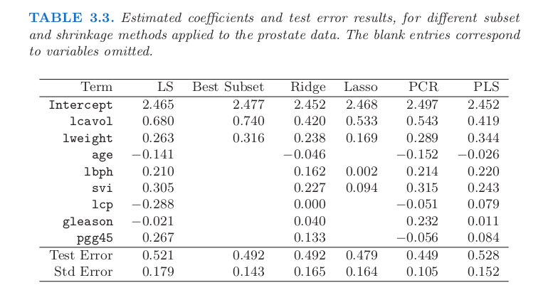
Warning: In the book is not provided the reg parameter choosen to perform Lasso for the table
The above chart is the figure 3.8 in the book The Elements of Statistical Learning: Data Mining, Inference, and Prediction. ↩︎