- Welcome to Congo! :tada:/
- Posts/
- Some exercise about Statistical Learning/
- SL5: Human Tumor Microarray dataset - clustering with k-means/
SL5: Human Tumor Microarray dataset - clustering with k-means
Table of Contents
# data analysis and wrangling
import numpy as np # linear algebra
import pandas as pd # data processing, CSV file I/O (e.g. pd.read_csv)
# import random as rnd

# visualization
import seaborn as sns
import matplotlib.pyplot as plt
# %matplotlib inline

# machine learning
from sklearn.cluster import KMeans
from sklearn.cluster import MiniBatchKMeans

from IPython.display import Image # to visualize images
from tabulate import tabulate # to create tables

import os
for dirname, _, filenames in os.walk('/kaggle/input'):
    for filename in filenames:
        print(os.path.join(dirname, filename))
/kaggle/input/14cancer/chart.png
/kaggle/input/14cancer/14cancer.ytrain.txt
/kaggle/input/14cancer/14cancer.xtrain.txt
/kaggle/input/14cancer/chart2.png
1. Download the “14-cancer microarray data” from the book website
- Get information about the dataset in file 14cancer.info and in Chapter 1 (page 5) of the book (Hastie et al., 2009)
Some info about 14cancer.xtrain.txt and14cancer.ytrain.txt.
DNA microarrays measure the expression of genes in a cell
14-cancer gene expression data set:
- 16064 genes
- 144 training samples
- 54 test samples
One gene per row, one sample per column.
Cancer classes are labelled as follows:
- breast
- prostate
- lung
- collerectal
- lymphoma
- bladder
- melanoma
- uterus
- leukemia
- renal
- pancreas
- ovary
- meso
- cns
2. Generate a new Kernel and give it the name:
“SL_EX5_HTM_Clustering_Surname”3. Load the data in Kaggle
Data acquisition #
# Load the Cancer Microarray dataset (already splitted in train and test)
xtrain = pd.read_csv('/kaggle/input/14cancer/14cancer.xtrain.txt', sep='\s+',header=None)
ytrain = pd.read_csv('/kaggle/input/14cancer/14cancer.ytrain.txt',sep='\s+',header=None)
Data pre-processing #
xtrain = xtrain.transpose() # The columns represent the genes, and the rows are the different samples
ytrain = ytrain.transpose() # for each sample I have a label

(n_samples, n_genes), n_labels = xtrain.shape, np.unique(ytrain).size
print(f"#genes: {n_genes}, #samples: {n_samples}, #labels {n_labels}")
#genes: 16063, #samples: 144, #labels 14
xtrain
| 0 | 1 | 2 | 3 | 4 | 5 | 6 | 7 | 8 | 9 | ... | 16053 | 16054 | 16055 | 16056 | 16057 | 16058 | 16059 | 16060 | 16061 | 16062 | |
|---|---|---|---|---|---|---|---|---|---|---|---|---|---|---|---|---|---|---|---|---|---|
| 0 | -73.0 | -69.0 | -48.0 | 13.0 | -86.0 | -147.0 | -65.0 | -71.0 | -32.0 | 100.0 | ... | -134.0 | 352.0 | -67.0 | 121.0 | -5.0 | -11.0 | -21.0 | -41.0 | -967.0 | -120.0 |
| 1 | -16.0 | -63.0 | -97.0 | -42.0 | -91.0 | -164.0 | -53.0 | -77.0 | -17.0 | 122.0 | ... | -51.0 | 244.0 | -15.0 | 119.0 | -32.0 | 4.0 | -14.0 | -28.0 | -205.0 | -31.0 |
| 2 | 4.0 | -45.0 | -112.0 | -25.0 | -85.0 | -127.0 | 56.0 | -110.0 | 81.0 | 41.0 | ... | 14.0 | 163.0 | -14.0 | 7.0 | 15.0 | -8.0 | -104.0 | -36.0 | -245.0 | 34.0 |
| 3 | -31.0 | -110.0 | -20.0 | -50.0 | -115.0 | -113.0 | -17.0 | -40.0 | -17.0 | 80.0 | ... | 26.0 | 625.0 | 18.0 | 59.0 | -10.0 | 32.0 | -2.0 | 10.0 | -495.0 | -37.0 |
| 4 | -33.0 | -39.0 | -45.0 | 14.0 | -56.0 | -106.0 | 73.0 | -34.0 | 18.0 | 64.0 | ... | -69.0 | 398.0 | 38.0 | 215.0 | -2.0 | 44.0 | 3.0 | 68.0 | -293.0 | -34.0 |
| ... | ... | ... | ... | ... | ... | ... | ... | ... | ... | ... | ... | ... | ... | ... | ... | ... | ... | ... | ... | ... | ... |
| 139 | -196.0 | -369.0 | -263.0 | 162.0 | -277.0 | -615.0 | -397.0 | -243.0 | 70.0 | -167.0 | ... | -25.0 | 2674.0 | 171.0 | 1499.0 | 95.0 | 735.0 | -12.0 | 647.0 | -2414.0 | -33.0 |
| 140 | 34.0 | -81.0 | -146.0 | -151.0 | -174.0 | -121.0 | -290.0 | -106.0 | 43.0 | 240.0 | ... | -32.0 | 226.0 | 189.0 | 310.0 | -13.0 | 210.0 | -22.0 | 622.0 | -889.0 | -104.0 |
| 141 | -56.0 | -818.0 | -1338.0 | -57.0 | -989.0 | -796.0 | -1466.0 | -347.0 | -413.0 | 103.0 | ... | -85.0 | 1827.0 | 581.0 | 1547.0 | -72.0 | 999.0 | -461.0 | 564.0 | -3567.0 | -192.0 |
| 142 | -245.0 | -235.0 | -127.0 | 197.0 | -562.0 | -714.0 | -1621.0 | -226.0 | -35.0 | -243.0 | ... | -419.0 | 580.0 | 233.0 | 1065.0 | -71.0 | 397.0 | -28.0 | 114.0 | -3086.0 | -16.0 |
| 143 | -26.0 | -1595.0 | -2085.0 | -334.0 | -455.0 | -354.0 | -482.0 | 196.0 | 114.0 | 45.0 | ... | -243.0 | 526.0 | 126.0 | 320.0 | -30.0 | 308.0 | -179.0 | 121.0 | -1878.0 | -357.0 |
144 rows × 16063 columns
Clustering Analysis #
4. Use thesklearn.cluster module to perform clustering analysis on the dataset. In particular, repeat the analysis proposed in section 14.3.8 of the book (Hastie et al., 2009)
- Start using
K-meansand then test some other clustering algorithms at your choice - Cluster the samples (i.e., columns). Each sample has a label (tumor type)
- Do not use the labels in the clustering phase but examine them posthoc to interpret the clusters
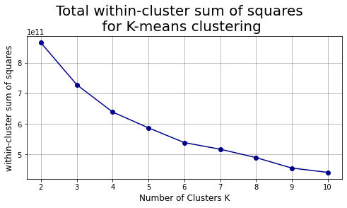
- Run k-means with K from 2 to 10 and compare the clusterings in terms of within-sum of squares
- Show the chart of the performance depending on K
- Select some K and analyze the clusters as done in the book
K-Means #
The KMeans algorithm clusters data by trying to separate samples in n groups of equal variance, minimizing a criterion known as the inertia or within-cluster sum-of-squares. 1
The k-means algorithm divides a set of samples into disjoint clusters, each described by the mean of the samples in the cluster. The means are commonly called the cluster “centroids”; note that they are not, in general, points from, although they live in the same space.
The K-means algorithm aims to choose centroids that minimise the inertia, or within-cluster sum-of-squares criterion: \[\sum_{i=0}^{n}\min_{\mu_j \in C}(||x_i - \mu_j||^2)\]
# K-means with k from 2 to 10

n_clusters = range(2,11)
alg = 'k-means++' # Method for initialization
niter = 10 # Number of time the k-means algorithm will be run with different centroid seeds.
wc_km_sos=[] # within_cluster_km_sos

print('k\tInertia\t\t\tdecrease %')
print(50 * '-')
formatter_result = ("{:d}\t{:f}\t{:f}")

for k in n_clusters:

    results = []
    results.append(k)

    km = KMeans(init=alg, n_clusters=k, n_init=niter).fit(xtrain)

    # inertia = Sum of squared distances of samples to their closest cluster center
    wcv = km.inertia_
    wc_km_sos.append(wcv)
    results.append(wcv)

    # variations in %
    if len(wc_km_sos)>1:
        results.append(
            (wc_km_sos[k-2] - wc_km_sos[k-3])*100/wc_km_sos[k-2]
        )
    else:
        results.append(0)

    print(formatter_result.format(*results))
k	Inertia			        decrease %
--------------------------------------------------
2	865755593329.079102 	0.000000
3	728028390816.590332	    -18.917834
4	638452947540.124023	    -14.030077
5	586449466492.984497	    -8.867513
6	538128754493.843750 	-8.979396
7	516487727616.067871 	-4.190037
8	488855618252.548340 	-5.652407
9	454592949466.325562	    -7.537000
10	440415484775.366333	    -3.219111
# fig
width, height = 8, 4
fig, ax = plt.subplots(figsize=(width,height))

ax.plot(n_clusters, wc_km_sos,  marker='o', color="darkblue")
ax.grid(color='grey', linestyle='-', linewidth=0.5);
#ax.yaxis.set_major_formatter(FormatStrFormatter('%.f'))

ax.set_xlabel("Number of Clusters K", fontsize=12)
ax.set_ylabel("within-cluster sum of squares", fontsize=12)

plt.suptitle("Total within-cluster sum of squares\n for K-means clustering",fontsize=20)
plt.subplots_adjust(top=0.825) # change title position

plt.show()
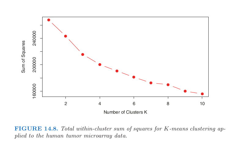
# We can compare the above chart with the one in the book:
scale = 80
Image("../input/14cancer/chart.png", width = width*scale, height = height*scale)
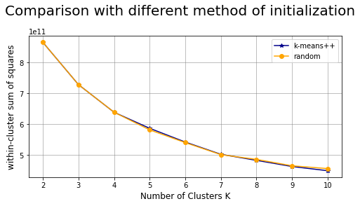
Comparison between different methods of initialization: k-means++ vs random #
n_clusters = range(2,11)
niter = 10 # Number of time the k-means algorithm will be run with different centroid seeds.
wc_kmpp, wc_rnd = [], []

print('k\tK-means\t\t\trandom')
print(60 * '-')
formatter_result = ("{:d}\t{:f}\t{:f}")

for k in n_clusters:

    results = []
    results.append(k)

    kmpp = KMeans(init="k-means++", n_clusters=k, n_init=niter).fit(xtrain)
    rnd = KMeans(init="random", n_clusters=k, n_init=niter).fit(xtrain)

    results.append(kmpp.inertia_)
    results.append(rnd.inertia_)

    wc_kmpp.append(kmpp.inertia_)
    wc_rnd.append(rnd.inertia_)

    print(formatter_result.format(*results))
k	K-means			        random
------------------------------------------------------------
2	865755593329.079102	    865755593329.078979
3	728215342983.054443	    728215342983.054443
4	638286863470.537109	    638452947540.124146
5	586098738159.229004	    580943572411.067993
6	541362331453.668213	    539591832514.661987
7	501565429046.019531	    500472648214.279541
8	481877683922.631714	    484882990782.917847
9	461806611237.345337	    464195618439.327515
10	448128965453.922974	    454970652718.346436
# fig
width, height = 8, 4
fig, ax = plt.subplots(figsize=(width,height))

ax.plot(n_clusters, wc_kmpp,  marker='*', color="darkblue", label = "k-means++")
ax.plot(n_clusters, wc_rnd,  marker='o', color="orange", label = "random")

ax.grid(color='grey', linestyle='-', linewidth=0.5);
#ax.yaxis.set_major_formatter(FormatStrFormatter('%.f'))
ax.legend()
ax.set_xlabel("Number of Clusters K", fontsize=12)
ax.set_ylabel("within-cluster sum of squares", fontsize=12)

plt.suptitle("Comparison with different method of initialization",fontsize=20)
plt.subplots_adjust(top=0.825) # change title position

plt.show()
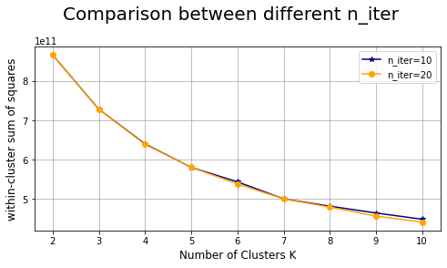
Comparison between different n_iter: #
Number of time the k-means algorithm will be run with different centroid seeds.
n_clusters = range(2,11)
wc_ten_seeds, wc_twenty_seeds = [], []

print('k\tn_iter=10\t\tn_iter=20')
print(70 * '-')
formatter_result = ("{:d}\t{:f}\t{:f}")

for k in n_clusters:

    results = []
    results.append(k)

    ten_seeds = KMeans(init="k-means++", n_clusters=k, n_init=10).fit(xtrain)
    twenty_seeds = KMeans(init="k-means++", n_clusters=k, n_init=20).fit(xtrain)

    results.append(ten_seeds.inertia_)
    results.append(twenty_seeds.inertia_)

    wc_ten_seeds.append(ten_seeds.inertia_)
    wc_twenty_seeds.append(twenty_seeds.inertia_)

    print(formatter_result.format(*results))
k	n_iter=10		        n_iter=20
----------------------------------------------------------------------
2	866070488704.476074	    865755593329.079102
3	728028390816.590210	    727972625271.491211
4	639723868185.660278 	638286863470.537109
5	579977474766.300903 	580224574540.047607
6	543140308602.200195 	537625894944.809998
7	499824352123.143555 	499900728332.191284
8	481177796841.305420 	478729684111.517700
9	463786737203.969238 	455823165084.713989
10	447920765947.759399 	440614709199.603394
# fig
width, height = 8, 4
fig, ax = plt.subplots(figsize=(width,height))

ax.plot(n_clusters, wc_ten_seeds,  marker='*', color="darkblue", label = "n_iter=10")
ax.plot(n_clusters, wc_twenty_seeds,  marker='o', color="orange", label = "n_iter=20")

ax.grid(color='grey', linestyle='-', linewidth=0.5);
#ax.yaxis.set_major_formatter(FormatStrFormatter('%.f'))
ax.legend()
ax.set_xlabel("Number of Clusters K", fontsize=12)
ax.set_ylabel("within-cluster sum of squares", fontsize=12)

plt.suptitle("Comparison between different n_iter",fontsize=20)
plt.subplots_adjust(top=0.825) # change title position

plt.show()
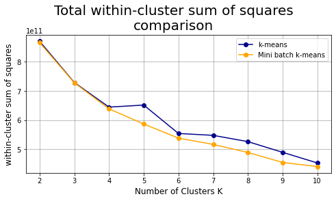
Mini-batch K-means #
The MiniBatchKMeans is a variant of the KMeans algorithm which uses mini-batches to reduce the computation time, while still attempting to optimise the same objective function.
Mini-batches are subsets of the input data, randomly sampled in each training iteration. These mini-batches drastically reduce the amount of computation required to converge to a local solution.
In contrast to other algorithms that reduce the convergence time of k-means, mini-batch k-means produces results that are generally only slightly worse than the standard algorithm. 1
# K-means with k from 2 to 10

n_clusters = range(2,11)
alg = 'k-means++' # Method for initialization
niter = 10 # Number of time the k-means algorithm will be run with different centroid seeds.
wc_mbkm_sos=[]

print('k\tInertia\t\t\tdecrease %')
print(50 * '-')
formatter_result = ("{:d}\t{:f}\t{:f}")

for k in n_clusters:

    results = []
    results.append(k)

    mbkm = MiniBatchKMeans(init=alg, n_clusters=k, n_init=niter).fit(xtrain)

    # inertia = Sum of squared distances of samples to their closest cluster center
    wcv = mbkm.inertia_
    wc_mbkm_sos.append(wcv)
    results.append(wcv)

    # variations in %
    if len(wc_mbkm_sos)>1:
        results.append(
            (wc_mbkm_sos[k-2] - wc_mbkm_sos[k-3])*100/wc_mbkm_sos[k-2]
        )
    else:
        results.append(0)

    print(formatter_result.format(*results))
k	Inertia			        decrease %
--------------------------------------------------
2	870435631688.268311	    0.000000
3	728979505913.590698	    -19.404678
4	644499761950.796875	    -13.107801
5	651489332987.863525	    1.072860
6	554034243741.206177	    -17.590084
7	547550479471.734985	    -1.184140
8	526030833538.899902	    -4.090948
9	489328464969.691284	    -7.500559
10	452845818672.533325	    -8.056306
# fig
width, height = 8, 4
fig, ax = plt.subplots(figsize=(width,height))

ax.plot(n_clusters, wc_mbkm_sos,  marker='o', color="darkblue", label = "k-means")
ax.plot(n_clusters, wc_km_sos,  marker='o', color="orange",  label = "Mini batch k-means")
ax.grid(color='grey', linestyle='-', linewidth=0.5);
#ax.yaxis.set_major_formatter(FormatStrFormatter('%.f'))

ax.legend()
ax.set_xlabel("Number of Clusters K", fontsize=12)
ax.set_ylabel("within-cluster sum of squares", fontsize=12)

plt.suptitle("Total within-cluster sum of squares\ncomparison",fontsize=20)
plt.subplots_adjust(top=0.825) # change title position

plt.show()
Analysis for K=3 #
Number of cancer cases of each type in each of the 3 clusters #
rows = KMeans(init="k-means++", n_clusters=3).fit(xtrain).labels_ # labels of each sample after clustering
columns = ytrain.to_numpy().flatten() # make the df into an iterable list

# Collect info in a table
tab = np.zeros(3*n_labels).reshape(3,n_labels) # rows: clusters, columns: cancer labels

# Update table
for i in range(n_samples):
    tab[rows[i],columns[i]-1]+=1 # column-1 because we range over 14 clusters (0,13)

# Better formatting of the table into a DataFrame
table = pd.DataFrame(tab.astype(int))
table.columns = ["breast", "prostate", "lung", "collerectal", "lymphoma", "bladder",
                 "melanoma", "uterus", "leukemia", "renal", "pancreas", "ovary", "meso", "cns"]
table
| breast | prostate | lung | collerectal | lymphoma | bladder | melanoma | uterus | leukemia | renal | pancreas | ovary | meso | cns | |
|---|---|---|---|---|---|---|---|---|---|---|---|---|---|---|
| 0 | 0 | 2 | 0 | 0 | 2 | 0 | 0 | 2 | 21 | 1 | 0 | 2 | 0 | 0 |
| 1 | 8 | 3 | 6 | 5 | 1 | 7 | 5 | 3 | 0 | 5 | 6 | 4 | 4 | 3 |
| 2 | 0 | 3 | 2 | 3 | 13 | 1 | 3 | 3 | 3 | 2 | 2 | 2 | 4 | 13 |
More info about K-Means method and other clustering methods can be found here ↩︎ ↩︎
The above chart can be found in the section 14.3.8 of the book The Elements of Statistical Learning: Data Mining, Inference, and Prediction. ↩︎