- Welcome to Congo! :tada:/
- Posts/
- Some exercise about Statistical Learning/
- SL6: California housing dataset – regression with ANN/
SL6: California housing dataset – regression with ANN
Table of Contents
# data analysis and wrangling
import numpy as np # linear algebra
import pandas as pd # data processing, CSV file I/O (e.g. pd.read_csv)
# import random as rnd

# visualization
import matplotlib.pyplot as plt
# %matplotlib inline

# machine learning
from sklearn.model_selection import train_test_split
import tensorflow as tf
from tensorflow import keras
from keras.models import  Sequential
from keras.layers.core import Dense
import keras.metrics as metrics


import os
for dirname, _, filenames in os.walk('/kaggle/input'):
    for filename in filenames:
        print(os.path.join(dirname, filename))
/kaggle/input/californiahousingdataset/train.csv
/kaggle/input/californiahousingdataset/test.csv
1. Browse the Keras library (tutorial and documentation cited in the slides)
2. Load the California housing dataset
Some info about the California_housing_dataset #
#samples-istances: 20640
variables: 8 numeric predictors, 1 target
- Predictors:
- MedInc (mi): median income in block
- HouseAge (ha): median house age in block
- AveRooms (ar): average number of rooms
- AveBedrms (ab): average number of bedrooms
- Population (p): block population
- AveOccup (ao): average house occupancy
- Latitude (lt): house block latitude
- Longitude (lg): house block longitude
- Response:
- Target (v): median house value for California districts
- Predictors:
Missing values: none
Data Acquisition #
# Load the California Housing dataset
df_train = pd.read_csv('../input/californiahousingdataset/train.csv',sep=',')
df_test = pd.read_csv('../input/californiahousingdataset/test.csv',sep=',')
# Some stats
print(f"We have {df_train.shape[0] + df_test.shape[0]} observation, splitted into:\n\
      * {df_train.shape[0]} training observations;\n\
      * {df_test.shape[0]} test observations.\n\
There are {df_train.isna().sum().sum() + df_test.isna().sum().sum()} missing values in the dataset.")
We have 20640 observation, splitted into:
      * 16385 training observations;
      * 4255 test observations.
There are 0 missing values in the dataset.
Data pre-processing #
# Drop an useless feature
df_train = df_train.drop(columns='Unnamed: 0');
df_test = df_test.drop(columns='Unnamed: 0');
df_train
| mi | ha | ar | ab | p | ao | lt | lg | v | |
|---|---|---|---|---|---|---|---|---|---|
| 0 | 5.8735 | 35.0 | 5.811639 | 1.056662 | 1521.0 | 2.329250 | 34.11 | -118.63 | 4.48100 |
| 1 | 1.4688 | 8.0 | 10.000000 | 1.916667 | 63.0 | 2.625000 | 33.32 | -115.98 | 0.53800 |
| 2 | 2.1603 | 28.0 | 4.808173 | 0.995460 | 2008.0 | 2.279228 | 38.74 | -120.78 | 1.11300 |
| 3 | 4.7404 | 43.0 | 5.855140 | 1.009346 | 967.0 | 2.259346 | 37.58 | -122.37 | 5.00001 |
| 4 | 3.2617 | 10.0 | 3.929142 | 1.051896 | 2032.0 | 2.027944 | 37.45 | -121.92 | 2.52200 |
| ... | ... | ... | ... | ... | ... | ... | ... | ... | ... |
| 16380 | 5.0427 | 22.0 | 6.405405 | 1.009828 | 1216.0 | 2.987715 | 38.55 | -121.35 | 1.26900 |
| 16381 | 4.7396 | 25.0 | 5.453390 | 0.949153 | 727.0 | 3.080508 | 38.73 | -121.44 | 1.35500 |
| 16382 | 5.0839 | 25.0 | 6.039216 | 1.150980 | 1558.0 | 3.054902 | 34.73 | -118.61 | 1.56700 |
| 16383 | 5.5292 | 16.0 | 6.875000 | 1.015086 | 1414.0 | 3.047414 | 34.11 | -117.68 | 2.08600 |
| 16384 | 5.1514 | 19.0 | 6.204918 | 1.001639 | 2198.0 | 3.603279 | 37.11 | -121.66 | 4.36700 |
16385 rows × 9 columns
Split the dataset into Training and Test sets #
# Training set
predictorsTrain = df_train.loc[:, df_train.columns != 'v']
responseTrain = df_train['v']

# Test set
predictorsTest = df_test.loc[:, df_train.columns != 'v']
responseTest = df_test['v']
Standardization #
# Standardize "predictorsTrain"
predictorsTrainMeans = predictorsTrain.mean()
predictorsTrainStds = predictorsTrain.std()
predictorsTrain_std = (predictorsTrain - predictorsTrainMeans)/predictorsTrainStds # standardized variables of predictorTrain

# Standardize "predictorsTest" (using the mean and std of predictorsTrain, it's better!)
predictorsTest_std = (predictorsTest - predictorsTrainMeans)/predictorsTrainStds # standardized variables of predictorTest
Split the training set into Train and Validation sets #
Splitting the dataset is essential for an unbiased evaluation of prediction performance. In most cases, it’s enough to split your dataset randomly into three subsets:
The training set is applied to train, or fit, your model. For example, you use the training set to find the optimal coefficients for linear regression.
The validation set is used for unbiased model evaluation during hyperparameter tuning. For example, when you want to find the optimal number of neurons in a neural network, you experiment with different values. For each considered setting of hyperparameters, you fit the model with the training set and assess its performance with the validation set.
The test set is needed for an unbiased evaluation of the final model. Don’t use it for fitting or validation.
I choosed to split the train set in two parts: a small fraction (20%) became the validation set which the model is evaluated and the rest (80%) is used to train the model.
# Set the random seed
random_seed = 3 # a random_state parameter may be provided to control the random number generator used
# Split the train and the validation set for the fitting
X_train, X_val, y_train, y_val = train_test_split(predictorsTrain_std, responseTrain, test_size = 0.2, random_state = random_seed)
X_train.shape, y_train.shape, X_val.shape, y_val.shape
((13108, 8), (13108,), (3277, 8), (3277,))
Rename the data
# Rename our data

## Training set - already done it above when I created the validation set
# X_train = X_train
# X_val = X_val
# y_train = y_train
# y_val = y_val

## Test set
X_test = predictorsTest_std
y_test = responseTest
# # Since Keras models are trained on Numpy arrays of input data and labels:

# # Training set
# # X_train = X_train.values
# # X_val = X_val.values
# # y_train = y_train.values
# # y_val = y_val.values

# # Test set
# X_test = X_test.values
# y_test = y_test.values
Generating the first Artificial Neural Network #
3. Generate the artificial neural network model analyzed in this slides and compare the results obtained by structures defined below**Create the ANN #
Lets create a simple model from Keras Sequential layer:
- Dense is fully connected layer that means all neurons in previous layers will be connected to all neurons in fully connected layer.
model = Sequential()

# Input Layer
model.add(Dense(10, input_dim=X_train.shape[1], activation='relu'))

# Hidden Layers
model.add(Dense(30, activation='relu'))
model.add(Dense(40, activation='relu'))

# Output Layer
model.add(Dense(1))
2022-06-24 16:09:21.913542: I tensorflow/core/common_runtime/process_util.cc:146] Creating new thread pool with default inter op setting: 2. Tune using inter_op_parallelism_threads for best performance.
Compile network #
# Compile the model
model.compile(optimizer ='adam',           # Optimizer: an algorithm for first-order stochastic gradiend descent
              loss = 'mean_squared_error', # Loss function: the objective that the model will try to minimize
              metrics=[metrics.mae])       # A list of metrics: used to judge the performance of your model
Fitting procedure #
EPOCHS = 150 # 150 are too much (using np.arrays)

print(f"Train on {X_train.shape[0]} samples, validate on {X_val.shape[0]} samples.")

# train model on full train set, with 80/20 CV split
history = model.fit(X_train, y_train,
                    validation_data=(X_val, y_val), # validation_data: data on which to evaluate the loss and any model metrics at the end of each epoch
                    epochs=EPOCHS,                  # epochs: number of iterations of the training phase
                    batch_size=32)                  # batch_size: number of samples per gradient update (default: 32)
Train on 13108 samples, validate on 3277 samples.
Epoch 1/150


2022-06-24 16:09:22.231798: I tensorflow/compiler/mlir/mlir_graph_optimization_pass.cc:185] None of the MLIR Optimization Passes are enabled (registered 2)


410/410 [==============================] - 2s 3ms/step - loss: 1.2253 - mean_absolute_error: 0.7533 - val_loss: 0.5908 - val_mean_absolute_error: 0.5529
Epoch 2/150
410/410 [==============================] - 1s 2ms/step - loss: 0.5182 - mean_absolute_error: 0.5102 - val_loss: 0.4717 - val_mean_absolute_error: 0.4867
Epoch 3/150
410/410 [==============================] - 1s 2ms/step - loss: 0.4256 - mean_absolute_error: 0.4662 - val_loss: 0.4313 - val_mean_absolute_error: 0.4772
Epoch 4/150
410/410 [==============================] - 1s 2ms/step - loss: 0.3909 - mean_absolute_error: 0.4474 - val_loss: 0.4028 - val_mean_absolute_error: 0.4475
Epoch 5/150
410/410 [==============================] - 1s 2ms/step - loss: 0.3738 - mean_absolute_error: 0.4374 - val_loss: 0.4008 - val_mean_absolute_error: 0.4341
Epoch 6/150
410/410 [==============================] - 1s 2ms/step - loss: 0.3637 - mean_absolute_error: 0.4284 - val_loss: 0.3835 - val_mean_absolute_error: 0.4412
Epoch 7/150
410/410 [==============================] - 1s 2ms/step - loss: 0.3578 - mean_absolute_error: 0.4246 - val_loss: 0.3987 - val_mean_absolute_error: 0.4290
Epoch 8/150
410/410 [==============================] - 1s 2ms/step - loss: 0.3471 - mean_absolute_error: 0.4180 - val_loss: 0.3797 - val_mean_absolute_error: 0.4406
Epoch 9/150
410/410 [==============================] - 1s 2ms/step - loss: 0.3449 - mean_absolute_error: 0.4167 - val_loss: 0.3776 - val_mean_absolute_error: 0.4168
Epoch 10/150
410/410 [==============================] - 1s 2ms/step - loss: 0.3375 - mean_absolute_error: 0.4114 - val_loss: 0.3777 - val_mean_absolute_error: 0.4179
Epoch 11/150
410/410 [==============================] - 1s 2ms/step - loss: 0.3341 - mean_absolute_error: 0.4091 - val_loss: 0.3913 - val_mean_absolute_error: 0.4518
Epoch 12/150
410/410 [==============================] - 1s 2ms/step - loss: 0.3310 - mean_absolute_error: 0.4078 - val_loss: 0.3635 - val_mean_absolute_error: 0.4131
Epoch 13/150
410/410 [==============================] - 1s 2ms/step - loss: 0.3272 - mean_absolute_error: 0.4033 - val_loss: 0.3650 - val_mean_absolute_error: 0.4186
Epoch 14/150
410/410 [==============================] - 1s 2ms/step - loss: 0.3244 - mean_absolute_error: 0.4007 - val_loss: 0.3560 - val_mean_absolute_error: 0.4127
Epoch 15/150
410/410 [==============================] - 1s 3ms/step - loss: 0.3186 - mean_absolute_error: 0.3977 - val_loss: 0.3796 - val_mean_absolute_error: 0.4072
Epoch 16/150
410/410 [==============================] - 1s 2ms/step - loss: 0.3209 - mean_absolute_error: 0.3966 - val_loss: 0.3632 - val_mean_absolute_error: 0.4107
Epoch 17/150
410/410 [==============================] - 1s 2ms/step - loss: 0.3142 - mean_absolute_error: 0.3922 - val_loss: 0.3457 - val_mean_absolute_error: 0.4125
Epoch 18/150
410/410 [==============================] - 1s 2ms/step - loss: 0.3075 - mean_absolute_error: 0.3894 - val_loss: 0.3431 - val_mean_absolute_error: 0.4050
Epoch 19/150
410/410 [==============================] - 1s 2ms/step - loss: 0.3045 - mean_absolute_error: 0.3875 - val_loss: 0.3506 - val_mean_absolute_error: 0.3960
Epoch 20/150
410/410 [==============================] - 1s 2ms/step - loss: 0.3029 - mean_absolute_error: 0.3854 - val_loss: 0.3421 - val_mean_absolute_error: 0.3993
Epoch 21/150
410/410 [==============================] - 1s 2ms/step - loss: 0.2997 - mean_absolute_error: 0.3831 - val_loss: 0.3396 - val_mean_absolute_error: 0.4012
Epoch 22/150
410/410 [==============================] - 1s 2ms/step - loss: 0.2966 - mean_absolute_error: 0.3803 - val_loss: 0.3392 - val_mean_absolute_error: 0.3958
Epoch 23/150
410/410 [==============================] - 1s 2ms/step - loss: 0.2966 - mean_absolute_error: 0.3804 - val_loss: 0.3374 - val_mean_absolute_error: 0.3996
Epoch 24/150
410/410 [==============================] - 1s 2ms/step - loss: 0.2963 - mean_absolute_error: 0.3801 - val_loss: 0.3317 - val_mean_absolute_error: 0.3929
Epoch 25/150
410/410 [==============================] - 1s 2ms/step - loss: 0.2920 - mean_absolute_error: 0.3767 - val_loss: 0.3299 - val_mean_absolute_error: 0.3868
Epoch 26/150
410/410 [==============================] - 1s 2ms/step - loss: 0.2890 - mean_absolute_error: 0.3742 - val_loss: 0.3314 - val_mean_absolute_error: 0.3980
Epoch 27/150
410/410 [==============================] - 1s 2ms/step - loss: 0.2916 - mean_absolute_error: 0.3773 - val_loss: 0.3312 - val_mean_absolute_error: 0.3837
Epoch 28/150
410/410 [==============================] - 1s 2ms/step - loss: 0.2870 - mean_absolute_error: 0.3721 - val_loss: 0.3285 - val_mean_absolute_error: 0.3937
Epoch 29/150
410/410 [==============================] - 1s 2ms/step - loss: 0.2873 - mean_absolute_error: 0.3722 - val_loss: 0.3345 - val_mean_absolute_error: 0.3871
Epoch 30/150
410/410 [==============================] - 1s 2ms/step - loss: 0.2849 - mean_absolute_error: 0.3716 - val_loss: 0.3309 - val_mean_absolute_error: 0.3861
Epoch 31/150
410/410 [==============================] - 1s 2ms/step - loss: 0.2825 - mean_absolute_error: 0.3690 - val_loss: 0.3465 - val_mean_absolute_error: 0.3935
Epoch 32/150
410/410 [==============================] - 1s 2ms/step - loss: 0.2835 - mean_absolute_error: 0.3703 - val_loss: 0.3266 - val_mean_absolute_error: 0.3992
Epoch 33/150
410/410 [==============================] - 1s 2ms/step - loss: 0.2816 - mean_absolute_error: 0.3679 - val_loss: 0.3259 - val_mean_absolute_error: 0.3915
Epoch 34/150
410/410 [==============================] - 1s 2ms/step - loss: 0.2785 - mean_absolute_error: 0.3664 - val_loss: 0.3205 - val_mean_absolute_error: 0.3787
Epoch 35/150
410/410 [==============================] - 1s 2ms/step - loss: 0.2790 - mean_absolute_error: 0.3660 - val_loss: 0.3246 - val_mean_absolute_error: 0.3951
Epoch 36/150
410/410 [==============================] - 1s 2ms/step - loss: 0.2759 - mean_absolute_error: 0.3640 - val_loss: 0.3227 - val_mean_absolute_error: 0.3902
Epoch 37/150
410/410 [==============================] - 1s 2ms/step - loss: 0.2759 - mean_absolute_error: 0.3632 - val_loss: 0.3226 - val_mean_absolute_error: 0.3959
Epoch 38/150
410/410 [==============================] - 1s 2ms/step - loss: 0.2734 - mean_absolute_error: 0.3623 - val_loss: 0.3232 - val_mean_absolute_error: 0.3744
Epoch 39/150
410/410 [==============================] - 1s 2ms/step - loss: 0.2699 - mean_absolute_error: 0.3584 - val_loss: 0.3181 - val_mean_absolute_error: 0.3905
Epoch 40/150
410/410 [==============================] - 1s 2ms/step - loss: 0.2707 - mean_absolute_error: 0.3593 - val_loss: 0.3274 - val_mean_absolute_error: 0.3990
Epoch 41/150
410/410 [==============================] - 1s 2ms/step - loss: 0.2704 - mean_absolute_error: 0.3592 - val_loss: 0.3200 - val_mean_absolute_error: 0.3748
Epoch 42/150
410/410 [==============================] - 1s 2ms/step - loss: 0.2685 - mean_absolute_error: 0.3592 - val_loss: 0.3129 - val_mean_absolute_error: 0.3802
Epoch 43/150
410/410 [==============================] - 1s 2ms/step - loss: 0.2676 - mean_absolute_error: 0.3571 - val_loss: 0.3128 - val_mean_absolute_error: 0.3720
Epoch 44/150
410/410 [==============================] - 1s 2ms/step - loss: 0.2670 - mean_absolute_error: 0.3563 - val_loss: 0.3225 - val_mean_absolute_error: 0.3992
Epoch 45/150
410/410 [==============================] - 1s 2ms/step - loss: 0.2645 - mean_absolute_error: 0.3547 - val_loss: 0.3103 - val_mean_absolute_error: 0.3783
Epoch 46/150
410/410 [==============================] - 1s 2ms/step - loss: 0.2649 - mean_absolute_error: 0.3549 - val_loss: 0.3098 - val_mean_absolute_error: 0.3795
Epoch 47/150
410/410 [==============================] - 1s 2ms/step - loss: 0.2635 - mean_absolute_error: 0.3545 - val_loss: 0.3124 - val_mean_absolute_error: 0.3750
Epoch 48/150
410/410 [==============================] - 1s 2ms/step - loss: 0.2651 - mean_absolute_error: 0.3544 - val_loss: 0.3114 - val_mean_absolute_error: 0.3776
Epoch 49/150
410/410 [==============================] - 1s 2ms/step - loss: 0.2622 - mean_absolute_error: 0.3524 - val_loss: 0.3091 - val_mean_absolute_error: 0.3770
Epoch 50/150
410/410 [==============================] - 1s 2ms/step - loss: 0.2624 - mean_absolute_error: 0.3526 - val_loss: 0.3110 - val_mean_absolute_error: 0.3730
Epoch 51/150
410/410 [==============================] - 1s 2ms/step - loss: 0.2588 - mean_absolute_error: 0.3497 - val_loss: 0.3087 - val_mean_absolute_error: 0.3704
Epoch 52/150
410/410 [==============================] - 1s 3ms/step - loss: 0.2628 - mean_absolute_error: 0.3516 - val_loss: 0.3232 - val_mean_absolute_error: 0.3949
Epoch 53/150
410/410 [==============================] - 1s 2ms/step - loss: 0.2598 - mean_absolute_error: 0.3493 - val_loss: 0.3068 - val_mean_absolute_error: 0.3712
Epoch 54/150
410/410 [==============================] - 1s 2ms/step - loss: 0.2577 - mean_absolute_error: 0.3476 - val_loss: 0.3082 - val_mean_absolute_error: 0.3790
Epoch 55/150
410/410 [==============================] - 1s 2ms/step - loss: 0.2569 - mean_absolute_error: 0.3483 - val_loss: 0.3132 - val_mean_absolute_error: 0.3695
Epoch 56/150
410/410 [==============================] - 1s 2ms/step - loss: 0.2563 - mean_absolute_error: 0.3479 - val_loss: 0.3023 - val_mean_absolute_error: 0.3664
Epoch 57/150
410/410 [==============================] - 1s 2ms/step - loss: 0.2538 - mean_absolute_error: 0.3458 - val_loss: 0.3114 - val_mean_absolute_error: 0.3833
Epoch 58/150
410/410 [==============================] - 1s 2ms/step - loss: 0.2532 - mean_absolute_error: 0.3450 - val_loss: 0.3077 - val_mean_absolute_error: 0.3813
Epoch 59/150
410/410 [==============================] - 1s 2ms/step - loss: 0.2536 - mean_absolute_error: 0.3451 - val_loss: 0.3078 - val_mean_absolute_error: 0.3684
Epoch 60/150
410/410 [==============================] - 1s 2ms/step - loss: 0.2531 - mean_absolute_error: 0.3446 - val_loss: 0.3080 - val_mean_absolute_error: 0.3695
Epoch 61/150
410/410 [==============================] - 1s 2ms/step - loss: 0.2529 - mean_absolute_error: 0.3440 - val_loss: 0.3052 - val_mean_absolute_error: 0.3708
Epoch 62/150
410/410 [==============================] - 1s 2ms/step - loss: 0.2518 - mean_absolute_error: 0.3435 - val_loss: 0.3037 - val_mean_absolute_error: 0.3703
Epoch 63/150
410/410 [==============================] - 1s 2ms/step - loss: 0.2515 - mean_absolute_error: 0.3437 - val_loss: 0.3066 - val_mean_absolute_error: 0.3735
Epoch 64/150
410/410 [==============================] - 1s 2ms/step - loss: 0.2524 - mean_absolute_error: 0.3442 - val_loss: 0.3064 - val_mean_absolute_error: 0.3790
Epoch 65/150
410/410 [==============================] - 1s 2ms/step - loss: 0.2499 - mean_absolute_error: 0.3423 - val_loss: 0.3079 - val_mean_absolute_error: 0.3698
Epoch 66/150
410/410 [==============================] - 1s 2ms/step - loss: 0.2503 - mean_absolute_error: 0.3431 - val_loss: 0.3095 - val_mean_absolute_error: 0.3662
Epoch 67/150
410/410 [==============================] - 1s 2ms/step - loss: 0.2479 - mean_absolute_error: 0.3408 - val_loss: 0.3021 - val_mean_absolute_error: 0.3635
Epoch 68/150
410/410 [==============================] - 1s 2ms/step - loss: 0.2493 - mean_absolute_error: 0.3419 - val_loss: 0.3027 - val_mean_absolute_error: 0.3623
Epoch 69/150
410/410 [==============================] - 1s 2ms/step - loss: 0.2488 - mean_absolute_error: 0.3414 - val_loss: 0.3055 - val_mean_absolute_error: 0.3688
Epoch 70/150
410/410 [==============================] - 1s 2ms/step - loss: 0.2480 - mean_absolute_error: 0.3406 - val_loss: 0.3127 - val_mean_absolute_error: 0.3661
Epoch 71/150
410/410 [==============================] - 1s 2ms/step - loss: 0.2481 - mean_absolute_error: 0.3394 - val_loss: 0.3071 - val_mean_absolute_error: 0.3783
Epoch 72/150
410/410 [==============================] - 1s 2ms/step - loss: 0.2502 - mean_absolute_error: 0.3414 - val_loss: 0.2998 - val_mean_absolute_error: 0.3706
Epoch 73/150
410/410 [==============================] - 1s 2ms/step - loss: 0.2475 - mean_absolute_error: 0.3403 - val_loss: 0.2979 - val_mean_absolute_error: 0.3608
Epoch 74/150
410/410 [==============================] - 1s 2ms/step - loss: 0.2443 - mean_absolute_error: 0.3377 - val_loss: 0.3053 - val_mean_absolute_error: 0.3644
Epoch 75/150
410/410 [==============================] - 1s 2ms/step - loss: 0.2479 - mean_absolute_error: 0.3394 - val_loss: 0.3181 - val_mean_absolute_error: 0.3924
Epoch 76/150
410/410 [==============================] - 1s 2ms/step - loss: 0.2457 - mean_absolute_error: 0.3392 - val_loss: 0.3049 - val_mean_absolute_error: 0.3735
Epoch 77/150
410/410 [==============================] - 1s 2ms/step - loss: 0.2435 - mean_absolute_error: 0.3374 - val_loss: 0.3039 - val_mean_absolute_error: 0.3625
Epoch 78/150
410/410 [==============================] - 1s 2ms/step - loss: 0.2449 - mean_absolute_error: 0.3389 - val_loss: 0.2987 - val_mean_absolute_error: 0.3651
Epoch 79/150
410/410 [==============================] - 1s 2ms/step - loss: 0.2439 - mean_absolute_error: 0.3386 - val_loss: 0.3043 - val_mean_absolute_error: 0.3621
Epoch 80/150
410/410 [==============================] - 1s 2ms/step - loss: 0.2427 - mean_absolute_error: 0.3368 - val_loss: 0.3064 - val_mean_absolute_error: 0.3756
Epoch 81/150
410/410 [==============================] - 1s 2ms/step - loss: 0.2428 - mean_absolute_error: 0.3360 - val_loss: 0.2989 - val_mean_absolute_error: 0.3723
Epoch 82/150
410/410 [==============================] - 1s 2ms/step - loss: 0.2414 - mean_absolute_error: 0.3351 - val_loss: 0.3052 - val_mean_absolute_error: 0.3797
Epoch 83/150
410/410 [==============================] - 1s 2ms/step - loss: 0.2424 - mean_absolute_error: 0.3364 - val_loss: 0.2976 - val_mean_absolute_error: 0.3585
Epoch 84/150
410/410 [==============================] - 1s 2ms/step - loss: 0.2410 - mean_absolute_error: 0.3353 - val_loss: 0.2986 - val_mean_absolute_error: 0.3675
Epoch 85/150
410/410 [==============================] - 1s 2ms/step - loss: 0.2416 - mean_absolute_error: 0.3352 - val_loss: 0.3049 - val_mean_absolute_error: 0.3712
Epoch 86/150
410/410 [==============================] - 1s 2ms/step - loss: 0.2417 - mean_absolute_error: 0.3344 - val_loss: 0.3122 - val_mean_absolute_error: 0.3806
Epoch 87/150
410/410 [==============================] - 1s 2ms/step - loss: 0.2417 - mean_absolute_error: 0.3353 - val_loss: 0.2922 - val_mean_absolute_error: 0.3573
Epoch 88/150
410/410 [==============================] - 1s 2ms/step - loss: 0.2402 - mean_absolute_error: 0.3347 - val_loss: 0.2990 - val_mean_absolute_error: 0.3648
Epoch 89/150
410/410 [==============================] - 1s 3ms/step - loss: 0.2383 - mean_absolute_error: 0.3324 - val_loss: 0.2984 - val_mean_absolute_error: 0.3653
Epoch 90/150
410/410 [==============================] - 1s 2ms/step - loss: 0.2397 - mean_absolute_error: 0.3338 - val_loss: 0.2947 - val_mean_absolute_error: 0.3648
Epoch 91/150
410/410 [==============================] - 1s 2ms/step - loss: 0.2402 - mean_absolute_error: 0.3341 - val_loss: 0.3147 - val_mean_absolute_error: 0.3704
Epoch 92/150
410/410 [==============================] - 1s 2ms/step - loss: 0.2391 - mean_absolute_error: 0.3340 - val_loss: 0.2971 - val_mean_absolute_error: 0.3636
Epoch 93/150
410/410 [==============================] - 1s 2ms/step - loss: 0.2379 - mean_absolute_error: 0.3323 - val_loss: 0.2973 - val_mean_absolute_error: 0.3563
Epoch 94/150
410/410 [==============================] - 1s 2ms/step - loss: 0.2369 - mean_absolute_error: 0.3320 - val_loss: 0.3061 - val_mean_absolute_error: 0.3600
Epoch 95/150
410/410 [==============================] - 1s 2ms/step - loss: 0.2367 - mean_absolute_error: 0.3320 - val_loss: 0.2945 - val_mean_absolute_error: 0.3626
Epoch 96/150
410/410 [==============================] - 1s 2ms/step - loss: 0.2374 - mean_absolute_error: 0.3332 - val_loss: 0.2952 - val_mean_absolute_error: 0.3661
Epoch 97/150
410/410 [==============================] - 1s 2ms/step - loss: 0.2360 - mean_absolute_error: 0.3314 - val_loss: 0.3027 - val_mean_absolute_error: 0.3579
Epoch 98/150
410/410 [==============================] - 1s 2ms/step - loss: 0.2370 - mean_absolute_error: 0.3329 - val_loss: 0.2946 - val_mean_absolute_error: 0.3585
Epoch 99/150
410/410 [==============================] - 1s 2ms/step - loss: 0.2401 - mean_absolute_error: 0.3325 - val_loss: 0.2981 - val_mean_absolute_error: 0.3572
Epoch 100/150
410/410 [==============================] - 1s 2ms/step - loss: 0.2350 - mean_absolute_error: 0.3313 - val_loss: 0.2998 - val_mean_absolute_error: 0.3569
Epoch 101/150
410/410 [==============================] - 1s 2ms/step - loss: 0.2348 - mean_absolute_error: 0.3308 - val_loss: 0.2981 - val_mean_absolute_error: 0.3718
Epoch 102/150
410/410 [==============================] - 1s 2ms/step - loss: 0.2332 - mean_absolute_error: 0.3292 - val_loss: 0.3151 - val_mean_absolute_error: 0.3881
Epoch 103/150
410/410 [==============================] - 1s 2ms/step - loss: 0.2338 - mean_absolute_error: 0.3298 - val_loss: 0.2954 - val_mean_absolute_error: 0.3628
Epoch 104/150
410/410 [==============================] - 1s 2ms/step - loss: 0.2336 - mean_absolute_error: 0.3298 - val_loss: 0.3009 - val_mean_absolute_error: 0.3679
Epoch 105/150
410/410 [==============================] - 1s 2ms/step - loss: 0.2329 - mean_absolute_error: 0.3289 - val_loss: 0.2938 - val_mean_absolute_error: 0.3587
Epoch 106/150
410/410 [==============================] - 1s 2ms/step - loss: 0.2316 - mean_absolute_error: 0.3283 - val_loss: 0.2990 - val_mean_absolute_error: 0.3556
Epoch 107/150
410/410 [==============================] - 1s 2ms/step - loss: 0.2329 - mean_absolute_error: 0.3291 - val_loss: 0.2904 - val_mean_absolute_error: 0.3553
Epoch 108/150
410/410 [==============================] - 1s 2ms/step - loss: 0.2321 - mean_absolute_error: 0.3277 - val_loss: 0.2956 - val_mean_absolute_error: 0.3588
Epoch 109/150
410/410 [==============================] - 1s 2ms/step - loss: 0.2353 - mean_absolute_error: 0.3298 - val_loss: 0.2900 - val_mean_absolute_error: 0.3645
Epoch 110/150
410/410 [==============================] - 1s 2ms/step - loss: 0.2321 - mean_absolute_error: 0.3289 - val_loss: 0.2951 - val_mean_absolute_error: 0.3708
Epoch 111/150
410/410 [==============================] - 1s 2ms/step - loss: 0.2292 - mean_absolute_error: 0.3267 - val_loss: 0.3024 - val_mean_absolute_error: 0.3787
Epoch 112/150
410/410 [==============================] - 1s 2ms/step - loss: 0.2297 - mean_absolute_error: 0.3265 - val_loss: 0.2942 - val_mean_absolute_error: 0.3593
Epoch 113/150
410/410 [==============================] - 1s 2ms/step - loss: 0.2305 - mean_absolute_error: 0.3275 - val_loss: 0.3016 - val_mean_absolute_error: 0.3767
Epoch 114/150
410/410 [==============================] - 1s 2ms/step - loss: 0.2281 - mean_absolute_error: 0.3264 - val_loss: 0.2936 - val_mean_absolute_error: 0.3552
Epoch 115/150
410/410 [==============================] - 1s 2ms/step - loss: 0.2295 - mean_absolute_error: 0.3273 - val_loss: 0.2995 - val_mean_absolute_error: 0.3701
Epoch 116/150
410/410 [==============================] - 1s 2ms/step - loss: 0.2286 - mean_absolute_error: 0.3263 - val_loss: 0.2912 - val_mean_absolute_error: 0.3616
Epoch 117/150
410/410 [==============================] - 1s 2ms/step - loss: 0.2287 - mean_absolute_error: 0.3257 - val_loss: 0.2982 - val_mean_absolute_error: 0.3655
Epoch 118/150
410/410 [==============================] - 1s 2ms/step - loss: 0.2297 - mean_absolute_error: 0.3258 - val_loss: 0.2932 - val_mean_absolute_error: 0.3663
Epoch 119/150
410/410 [==============================] - 1s 2ms/step - loss: 0.2282 - mean_absolute_error: 0.3254 - val_loss: 0.2913 - val_mean_absolute_error: 0.3551
Epoch 120/150
410/410 [==============================] - 1s 2ms/step - loss: 0.2289 - mean_absolute_error: 0.3261 - val_loss: 0.2969 - val_mean_absolute_error: 0.3529
Epoch 121/150
410/410 [==============================] - 1s 2ms/step - loss: 0.2273 - mean_absolute_error: 0.3247 - val_loss: 0.2998 - val_mean_absolute_error: 0.3777
Epoch 122/150
410/410 [==============================] - 1s 2ms/step - loss: 0.2274 - mean_absolute_error: 0.3261 - val_loss: 0.2891 - val_mean_absolute_error: 0.3607
Epoch 123/150
410/410 [==============================] - 1s 2ms/step - loss: 0.2295 - mean_absolute_error: 0.3272 - val_loss: 0.2906 - val_mean_absolute_error: 0.3588
Epoch 124/150
410/410 [==============================] - 1s 2ms/step - loss: 0.2290 - mean_absolute_error: 0.3273 - val_loss: 0.2894 - val_mean_absolute_error: 0.3602
Epoch 125/150
410/410 [==============================] - 1s 3ms/step - loss: 0.2278 - mean_absolute_error: 0.3256 - val_loss: 0.2883 - val_mean_absolute_error: 0.3590
Epoch 126/150
410/410 [==============================] - 1s 2ms/step - loss: 0.2269 - mean_absolute_error: 0.3252 - val_loss: 0.2937 - val_mean_absolute_error: 0.3556
Epoch 127/150
410/410 [==============================] - 1s 2ms/step - loss: 0.2271 - mean_absolute_error: 0.3246 - val_loss: 0.2919 - val_mean_absolute_error: 0.3541
Epoch 128/150
410/410 [==============================] - 1s 2ms/step - loss: 0.2256 - mean_absolute_error: 0.3242 - val_loss: 0.2894 - val_mean_absolute_error: 0.3544
Epoch 129/150
410/410 [==============================] - 1s 2ms/step - loss: 0.2248 - mean_absolute_error: 0.3242 - val_loss: 0.2890 - val_mean_absolute_error: 0.3536
Epoch 130/150
410/410 [==============================] - 1s 2ms/step - loss: 0.2258 - mean_absolute_error: 0.3251 - val_loss: 0.2888 - val_mean_absolute_error: 0.3498
Epoch 131/150
410/410 [==============================] - 1s 2ms/step - loss: 0.2267 - mean_absolute_error: 0.3249 - val_loss: 0.2890 - val_mean_absolute_error: 0.3571
Epoch 132/150
410/410 [==============================] - 1s 2ms/step - loss: 0.2255 - mean_absolute_error: 0.3225 - val_loss: 0.2959 - val_mean_absolute_error: 0.3639
Epoch 133/150
410/410 [==============================] - 1s 2ms/step - loss: 0.2247 - mean_absolute_error: 0.3238 - val_loss: 0.3008 - val_mean_absolute_error: 0.3538
Epoch 134/150
410/410 [==============================] - 1s 2ms/step - loss: 0.2256 - mean_absolute_error: 0.3236 - val_loss: 0.2906 - val_mean_absolute_error: 0.3499
Epoch 135/150
410/410 [==============================] - 1s 2ms/step - loss: 0.2233 - mean_absolute_error: 0.3225 - val_loss: 0.2922 - val_mean_absolute_error: 0.3584
Epoch 136/150
410/410 [==============================] - 1s 2ms/step - loss: 0.2223 - mean_absolute_error: 0.3218 - val_loss: 0.2916 - val_mean_absolute_error: 0.3576
Epoch 137/150
410/410 [==============================] - 1s 2ms/step - loss: 0.2224 - mean_absolute_error: 0.3210 - val_loss: 0.3019 - val_mean_absolute_error: 0.3587
Epoch 138/150
410/410 [==============================] - 1s 2ms/step - loss: 0.2238 - mean_absolute_error: 0.3229 - val_loss: 0.3015 - val_mean_absolute_error: 0.3580
Epoch 139/150
410/410 [==============================] - 1s 2ms/step - loss: 0.2238 - mean_absolute_error: 0.3229 - val_loss: 0.2901 - val_mean_absolute_error: 0.3607
Epoch 140/150
410/410 [==============================] - 1s 2ms/step - loss: 0.2248 - mean_absolute_error: 0.3239 - val_loss: 0.2936 - val_mean_absolute_error: 0.3643
Epoch 141/150
410/410 [==============================] - 1s 2ms/step - loss: 0.2237 - mean_absolute_error: 0.3225 - val_loss: 0.2952 - val_mean_absolute_error: 0.3576
Epoch 142/150
410/410 [==============================] - 1s 2ms/step - loss: 0.2227 - mean_absolute_error: 0.3218 - val_loss: 0.2827 - val_mean_absolute_error: 0.3479
Epoch 143/150
410/410 [==============================] - 1s 2ms/step - loss: 0.2221 - mean_absolute_error: 0.3203 - val_loss: 0.2915 - val_mean_absolute_error: 0.3605
Epoch 144/150
410/410 [==============================] - 1s 2ms/step - loss: 0.2232 - mean_absolute_error: 0.3222 - val_loss: 0.2929 - val_mean_absolute_error: 0.3605
Epoch 145/150
410/410 [==============================] - 1s 2ms/step - loss: 0.2223 - mean_absolute_error: 0.3216 - val_loss: 0.2914 - val_mean_absolute_error: 0.3639
Epoch 146/150
410/410 [==============================] - 1s 2ms/step - loss: 0.2225 - mean_absolute_error: 0.3235 - val_loss: 0.2891 - val_mean_absolute_error: 0.3572
Epoch 147/150
410/410 [==============================] - 1s 2ms/step - loss: 0.2214 - mean_absolute_error: 0.3210 - val_loss: 0.2862 - val_mean_absolute_error: 0.3535
Epoch 148/150
410/410 [==============================] - 1s 2ms/step - loss: 0.2221 - mean_absolute_error: 0.3216 - val_loss: 0.2944 - val_mean_absolute_error: 0.3589
Epoch 149/150
410/410 [==============================] - 1s 2ms/step - loss: 0.2235 - mean_absolute_error: 0.3226 - val_loss: 0.2892 - val_mean_absolute_error: 0.3554
Epoch 150/150
410/410 [==============================] - 1s 2ms/step - loss: 0.2205 - mean_absolute_error: 0.3197 - val_loss: 0.2908 - val_mean_absolute_error: 0.3615
print(
'- Stats on Training set:',
'\n\t* Loss:\t\t', history.history['loss'][-1],
'\n\t* MAE:\t\t', history.history['mean_absolute_error'][-1],
'\n- Stats on Validation set:',
'\n\t* loss:\t\t', history.history['val_loss'][-1],
'\n\t* MAE:\t\t', history.history['val_mean_absolute_error'][-1],
)
- Stats on Training set:
	* Loss:		 0.2204761952161789
	* MAE:		 0.3197171688079834
- Stats on Validation set:
	* loss:		 0.29083022475242615
	* MAE:		 0.3615073263645172
model.summary()
Model: "sequential"
_________________________________________________________________
Layer (type)                 Output Shape              Param #
=================================================================
dense (Dense)                (None, 10)                90
_________________________________________________________________
dense_1 (Dense)              (None, 30)                330
_________________________________________________________________
dense_2 (Dense)              (None, 40)                1240
_________________________________________________________________
dense_3 (Dense)              (None, 1)                 41
=================================================================
Total params: 1,701
Trainable params: 1,701
Non-trainable params: 0
_________________________________________________________________
From this observation, the formula seems to be: $$\#param = \#inp \cdot \#neurons_{layer_1};$$ but the true formula is: $$ \#param = (\#inp + 1) \cdot \#neurons_{layer_1}. $$ Maybe in the slides we have that #inputs = 7. 1
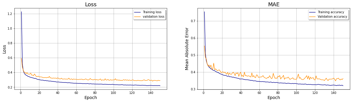
Evaluate the model #
On the Training set #
# Initialize the figure
width, height = 10, 5
nfig = 2
fig = plt.figure(figsize = (width*nfig,height))


# SBP 1: LOSS

ax1 = fig.add_subplot(1, nfig, 1);
ax1.plot(range(1,EPOCHS+1),history.history['loss'], color='darkblue', label="Training loss")
ax1.plot(range(1,EPOCHS+1),history.history['val_loss'], color='darkorange', label="validation loss",axes =ax1)

ax1.legend(loc='best', shadow=True)
ax1.set_xlabel('Epoch',fontsize=14);
ax1.set_ylabel('Loss',fontsize=14);
ax1.set_title('Loss',fontsize=18);
ax1.grid(color='grey', linestyle='-', linewidth=0.5);


# SBP 1: MAE

ax2 = fig.add_subplot(1, nfig, 2);
ax2.plot(range(1,EPOCHS+1),history.history['mean_absolute_error'], color='darkblue', label="Training accuracy")
ax2.plot(range(1,EPOCHS+1),history.history['val_mean_absolute_error'], color='darkorange',label="Validation accuracy")

ax2.legend(loc='best', shadow=True)
ax2.set_xlabel('Epoch',fontsize=14);
ax2.set_ylabel('Mean Absolute Error',fontsize=14);
ax2.set_title('MAE',fontsize=18);
ax2.grid(color='grey', linestyle='-', linewidth=0.5);

# plt.suptitle("Stats on Training set",fontsize=25)
# plt.subplots_adjust(top=0.8) # change title position

plt.show()
On the Test set #
def root_mean_squared_error(y_true, y_pred):
        return  np.sqrt(np.mean((y_pred-y_true)**2))
# Compute LOSS and MAE on Test set
loss, mae = model.evaluate(X_test, y_test, verbose = 0); # 133/133 because it's the number of batches:
                                                                   # X_test.shape[0]/32 (default batch_size = 32)
# Compute RMSE on Test set
y_pred = model.predict(X_test)

A = y_test.values     # convert into a numpy array
B = y_pred.flatten()  # to get rid off the multiple brackets returned by predict method

rmse = root_mean_squared_error(A, B)
print(f"- Statistics on the Test set:\n\
\t* Test Loss: {loss}\n\
\t* Test MAE: {mae}\n\
\t* Test RMSE: {rmse}"
)
- Statistics on the Test set:
	* Test Loss: 0.2790662944316864
	* Test MAE: 0.35706254839897156
	* Test RMSE: 0.5282672929159882
Generating other ANN models #
4. Test the following network structures and compare the results in terms of training/validation MAE/loss, RMSE on test set:
- 1 layer containing a single neuron
- 1 layer containing 3 neurons
- 1 layer containing 10 neurons
- 2 layers containing respectively 10 and 30 neurons
- 3 layers containing respectively 10, 30 and 40 neurons
def create_model(network):

    num_layers = len(network)

    model = Sequential()

    # Input Layer
    model.add(Dense(network[0], input_dim=X_train.shape[1], activation='relu'))

    # Hidden Layers
    if num_layers > 1:
        for i in range(1,num_layers):
            model.add(Dense(network[i], activation='relu'))

    # Output Layer
    model.add(Dense(1))

    return model
def get_test_stats(model, xtest, ytest, verbose_flag):

    # Compute LOSS and MAE on Test set
    loss, mae = model.evaluate(xtest, ytest, verbose = verbose_flag);

    # Compute RMSE on Test set
    y_pred = model.predict(xtest)
    rmse = root_mean_squared_error(y_test.values, y_pred.flatten())

    return loss, mae, rmse, y_pred
DOE = [[1], [3], [10], [10,30], [10,30,40]] #Design of experiment
from time import time

# Store the info in order to compare the results with the following models.
training_loss, training_MAE = [], []
val_loss, val_MAE = [], []
test_loss, test_MAE, test_RMSE = [], [], []
net_struct, net_epochs, pred_list = [], [], [] #info about the network setting

print(f"Now we preform {len(DOE)} ANN models.\n")

for network in DOE:

    idx = DOE.index(network) # we consider as "MODEL #0" the one shown above!

    print(150*"=")
    print(f"[INFO] MODEL #{idx+1} using {DOE[idx]} neurons. [{idx+1}/{len(DOE)}]\n")
    custom_model = create_model(network)

    ## Compile the model
    custom_model.compile(optimizer ='adam',loss = 'mean_squared_error', metrics=[metrics.mae])

    ## Train model on full train set, with 80/20 CV split
    print(f"[INFO] Fitting using {EPOCHS} epochs...")
    print(f"Train on {X_train.shape[0]} samples, validate on {X_val.shape[0]} samples.")
    tstart = time()
    custom_history = custom_model.fit(X_train, y_train,
                        validation_data=(X_val, y_val),
                        epochs=EPOCHS,
                        batch_size=32,
                        verbose = 0)
    tend = time() - tstart
    print(f"\n...OK, fitted the model in {tend}s.")

    ## Summary
    print("\n[INFO] Summary:")
    custom_model.summary()

    ## Test set statistics
    print("\n[INFO] Evaluate the model on Test set:")
    loss, mae, rmse, y_pred = get_test_stats(custom_model, X_test, y_test, verbose_flag = 1)

    print('\n[INFO] Statistics:\
\n- Stats on Training set:',
'\n\t* Loss:\t\t', custom_history.history['loss'][-1],
'\n\t* MAE:\t\t', custom_history.history['mean_absolute_error'][-1],
'\n- Stats on Validation set:',
'\n\t* loss:\t\t', custom_history.history['val_loss'][-1],
'\n\t* MAE:\t\t', custom_history.history['val_mean_absolute_error'][-1],
'\n- Stats on Test set:',
'\n\t* loss:\t\t', loss,
'\n\t* MAE:\t\t', mae,
'\n\t* RMSE:\t\t', rmse,
    )

    ## Store all the statistics
    # store training info
    training_loss.append(custom_history.history['loss'])
    training_MAE.append(custom_history.history['mean_absolute_error'])

    # store val info
    val_loss.append(custom_history.history['val_loss'])
    val_MAE.append(custom_history.history['val_mean_absolute_error'])

    # store test info
    test_loss.append(loss)
    test_MAE.append(mae)
    test_RMSE.append(rmse)


    #structure of the network
    net_struct.append(DOE[idx])
    net_epochs.append(EPOCHS)
    pred_list.append(y_pred)

    print(150*"=")
    print("\n")

print(f"Performed all the {len(DOE)} models.")
Now we preform 5 ANN models.

======================================================================================================================================================
[INFO] MODEL #1 using [1] neurons. [1/5]

[INFO] Fitting using 150 epochs...
Train on 13108 samples, validate on 3277 samples.

...OK, fitted the model in 81.33795595169067s.

[INFO] Summary:
Model: "sequential_1"
_________________________________________________________________
Layer (type)                 Output Shape              Param #
=================================================================
dense_4 (Dense)              (None, 1)                 9
_________________________________________________________________
dense_5 (Dense)              (None, 1)                 2
=================================================================
Total params: 11
Trainable params: 11
Non-trainable params: 0
_________________________________________________________________

[INFO] Evaluate the model on Test set:
133/133 [==============================] - 0s 1ms/step - loss: 0.5043 - mean_absolute_error: 0.5226

[INFO] Statistics:
- Stats on Training set:
	* Loss:		 0.5019071698188782
	* MAE:		 0.5186200737953186
- Stats on Validation set:
	* loss:		 0.5074825882911682
	* MAE:		 0.5189610123634338
- Stats on Test set:
	* loss:		 0.5042912364006042
	* MAE:		 0.5225676894187927
	* RMSE:		 0.7101348192496855
======================================================================================================================================================


======================================================================================================================================================
[INFO] MODEL #2 using [3] neurons. [2/5]

[INFO] Fitting using 150 epochs...
Train on 13108 samples, validate on 3277 samples.

...OK, fitted the model in 86.69740176200867s.

[INFO] Summary:
Model: "sequential_2"
_________________________________________________________________
Layer (type)                 Output Shape              Param #
=================================================================
dense_6 (Dense)              (None, 3)                 27
_________________________________________________________________
dense_7 (Dense)              (None, 1)                 4
=================================================================
Total params: 31
Trainable params: 31
Non-trainable params: 0
_________________________________________________________________

[INFO] Evaluate the model on Test set:
133/133 [==============================] - 0s 1ms/step - loss: 0.4569 - mean_absolute_error: 0.4864

[INFO] Statistics:
- Stats on Training set:
	* Loss:		 0.45196104049682617
	* MAE:		 0.4827933609485626
- Stats on Validation set:
	* loss:		 0.4575823247432709
	* MAE:		 0.4799402058124542
- Stats on Test set:
	* loss:		 0.4569326639175415
	* MAE:		 0.4863855540752411
	* RMSE:		 0.6759679391200216
======================================================================================================================================================


======================================================================================================================================================
[INFO] MODEL #3 using [10] neurons. [3/5]

[INFO] Fitting using 150 epochs...
Train on 13108 samples, validate on 3277 samples.

...OK, fitted the model in 85.105064868927s.

[INFO] Summary:
Model: "sequential_3"
_________________________________________________________________
Layer (type)                 Output Shape              Param #
=================================================================
dense_8 (Dense)              (None, 10)                90
_________________________________________________________________
dense_9 (Dense)              (None, 1)                 11
=================================================================
Total params: 101
Trainable params: 101
Non-trainable params: 0
_________________________________________________________________

[INFO] Evaluate the model on Test set:
133/133 [==============================] - 0s 1ms/step - loss: 0.3562 - mean_absolute_error: 0.4191

[INFO] Statistics:
- Stats on Training set:
	* Loss:		 0.3352857232093811
	* MAE:		 0.40571486949920654
- Stats on Validation set:
	* loss:		 0.36747753620147705
	* MAE:		 0.41564399003982544
- Stats on Test set:
	* loss:		 0.35619547963142395
	* MAE:		 0.4191289246082306
	* RMSE:		 0.59682117017886
======================================================================================================================================================


======================================================================================================================================================
[INFO] MODEL #4 using [10, 30] neurons. [4/5]

[INFO] Fitting using 150 epochs...
Train on 13108 samples, validate on 3277 samples.

...OK, fitted the model in 106.76856350898743s.

[INFO] Summary:
Model: "sequential_4"
_________________________________________________________________
Layer (type)                 Output Shape              Param #
=================================================================
dense_10 (Dense)             (None, 10)                90
_________________________________________________________________
dense_11 (Dense)             (None, 30)                330
_________________________________________________________________
dense_12 (Dense)             (None, 1)                 31
=================================================================
Total params: 451
Trainable params: 451
Non-trainable params: 0
_________________________________________________________________

[INFO] Evaluate the model on Test set:
133/133 [==============================] - 0s 1ms/step - loss: 0.2938 - mean_absolute_error: 0.3772

[INFO] Statistics:
- Stats on Training set:
	* Loss:		 0.25864139199256897
	* MAE:		 0.3488193154335022
- Stats on Validation set:
	* loss:		 0.29905804991722107
	* MAE:		 0.37346842885017395
- Stats on Test set:
	* loss:		 0.29382142424583435
	* MAE:		 0.37718966603279114
	* RMSE:		 0.5420530397809932
======================================================================================================================================================


======================================================================================================================================================
[INFO] MODEL #5 using [10, 30, 40] neurons. [5/5]

[INFO] Fitting using 150 epochs...
Train on 13108 samples, validate on 3277 samples.

...OK, fitted the model in 123.2047529220581s.

[INFO] Summary:
Model: "sequential_5"
_________________________________________________________________
Layer (type)                 Output Shape              Param #
=================================================================
dense_13 (Dense)             (None, 10)                90
_________________________________________________________________
dense_14 (Dense)             (None, 30)                330
_________________________________________________________________
dense_15 (Dense)             (None, 40)                1240
_________________________________________________________________
dense_16 (Dense)             (None, 1)                 41
=================================================================
Total params: 1,701
Trainable params: 1,701
Non-trainable params: 0
_________________________________________________________________

[INFO] Evaluate the model on Test set:
133/133 [==============================] - 0s 2ms/step - loss: 0.2787 - mean_absolute_error: 0.3495

[INFO] Statistics:
- Stats on Training set:
	* Loss:		 0.234622061252594
	* MAE:		 0.33155113458633423
- Stats on Validation set:
	* loss:		 0.2967351973056793
	* MAE:		 0.35640445351600647
- Stats on Test set:
	* loss:		 0.27867719531059265
	* MAE:		 0.3495338559150696
	* RMSE:		 0.5278987847617789
======================================================================================================================================================


Performed all the 5 models.
# Collect all the most useful data into a DataFrame
stats = pd.DataFrame({
    'ANN_structure': net_struct,
    'ANN_epochs': net_epochs,
    'Training Loss': [last for *_, last in training_loss],
    'Training MAE': [last for *_, last in training_MAE],
    'Validation Loss': [last for *_, 0.435833last in val_loss],
    'Validation MAE': [last for *_, last in val_MAE],
    'Test Loss': test_loss,
    'Test MAE': test_MAE,
    'Test RMSE': test_RMSE
})
stats
| ANN_structure | ANN_epochs | Training Loss | Training MAE | Validation Loss | Validation MAE | Test Loss | Test MAE | Test RMSE | |
|---|---|---|---|---|---|---|---|---|---|
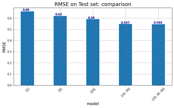
| 0 | [1] | 150 | 0.421746 | 0.471426 | 0.454049 | 0.483403 | 0.435833 | 0.480550 | 0.660177 |
| 1 | [3] | 150 | 0.372986 | 0.437562 | 0.405804 | 0.448418 | 0.384103 | 0.451114 | 0.619760 |
| 2 | [10] | 150 | 0.319872 | 0.398626 | 0.359499 | 0.417824 | 0.348028 | 0.418218 | 0.589939 |
| 3 | [10, 30] | 150 | 0.261056 | 0.350203 | 0.307047 | 0.368865 | 0.299178 | 0.371206 | 0.546971 |
| 4 | [10, 30, 40] | 150 | 0.239802 | 0.333529 | 0.308254 | 0.359592 | 0.298137 | 0.361128 | 0.546019 |
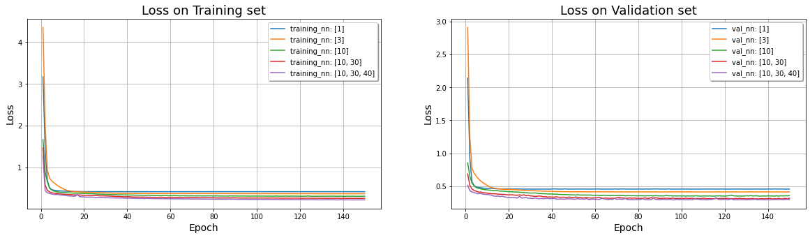
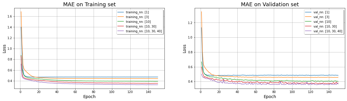
5. Generate a chart in which the performance of these models are displayed and compared
Compare the results #
On the Training set #
# Initialize the figure
width, height = 10, 5
nfig = 2
fig = plt.figure(figsize = (width*nfig,height))


# SBP 1: LOSS on Training set
ax1 = fig.add_subplot(1, nfig, 1);
for i in range(0,len(DOE)):
    ax1.plot(range(1,EPOCHS+1), training_loss[i], label="training_nn: " + str(net_struct[i]))
ax1.legend(loc='best', shadow=True)
ax1.set_xlabel('Epoch',fontsize=14);
ax1.set_ylabel('Loss',fontsize=14);
ax1.set_title('Loss on Training set',fontsize=18);
ax1.grid(color='grey', linestyle='-', linewidth=0.5);

# SBP 2: LOSS on Validation set
ax2 = fig.add_subplot(1, nfig, 2);
for i in range(0,len(DOE)):
    ax2.plot(range(1,EPOCHS+1), val_loss[i], label="val_nn: " + str(net_struct[i]))
ax2.legend(loc='best', shadow=True)
ax2.set_xlabel('Epoch',fontsize=14);
ax2.set_ylabel('Loss',fontsize=14);
ax2.set_title('Loss on Validation set',fontsize=18);
ax2.grid(color='grey', linestyle='-', linewidth=0.5);

plt.show()
# Initialize the figure
width, height = 10, 5
nfig = 2
fig = plt.figure(figsize = (width*nfig,height))


# SBP 1: LOSS on Training set
ax1 = fig.add_subplot(1, nfig, 1);
for i in range(0,len(DOE)):
    ax1.plot(range(1,EPOCHS+1), training_MAE[i], label="training_nn: " + str(net_struct[i]))
ax1.legend(loc='best', shadow=True)
ax1.set_xlabel('Epoch',fontsize=14);
ax1.set_ylabel('Loss',fontsize=14);
ax1.set_title('MAE on Training set',fontsize=18);
ax1.grid(color='grey', linestyle='-', linewidth=0.5);

# SBP 2: LOSS on Validation set
ax2 = fig.add_subplot(1, nfig, 2);
for i in range(0,len(DOE)):
    ax2.plot(range(1,EPOCHS+1), val_MAE[i], label="val_nn: " + str(net_struct[i]))
ax2.legend(loc='best', shadow=True)
ax2.set_xlabel('Epoch',fontsize=14);
ax2.set_ylabel('Loss',fontsize=14);
ax2.set_title('MAE on Validation set',fontsize=18);
ax2.grid(color='grey', linestyle='-', linewidth=0.5);

plt.show()
On the Test set #
# Initialize the figure
width, height = 10, 5
fig = plt.figure(figsize = (width,height))

ax1 = fig.add_subplot(1, 1, 1);
ax1.bar(range(1,len(DOE)+1), test_RMSE,width=0.4)

ax1.set_xlabel('model',fontsize=14);
ax1.set_ylabel('RMSE',fontsize=14);
ax1.set_title('RMSE on Test set: comparison',fontsize=18);
ax1.grid(color='grey', linestyle='-', linewidth=0.5);

# change the x-axis
xrange = [1,2,3,4,5]
squad = net_struct
ax1.set_xticks(xrange)
ax1.set_xticklabels(squad, minor=False, rotation=45)

for xx,yy in zip(xrange,test_RMSE):
    ax1.text(xx -0.15, yy + .005, str(test_RMSE[xx-1].round(3)), color='darkblue', fontweight='bold')


plt.show()
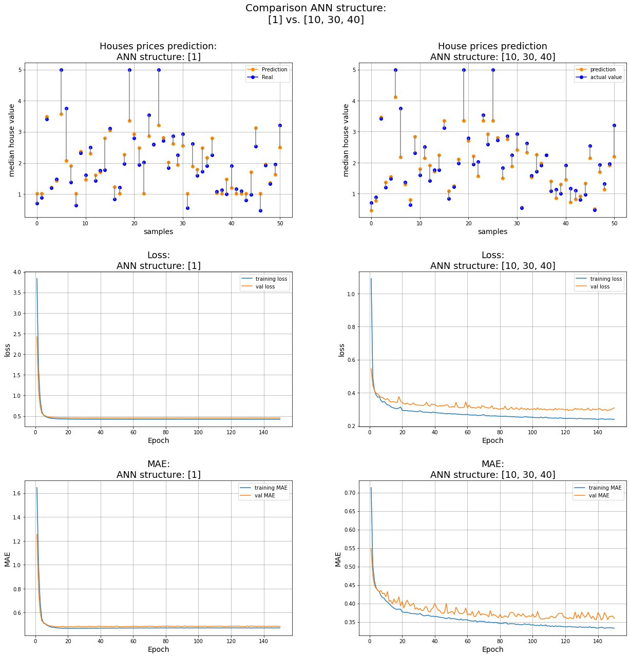
The first and the last models #
ns = 50 # number of samples to visualize
id_one, id_two = 0,-1 # index of the two models we want to compare

# Initialize the figure
width, height = 7, 10 # single pic
rows, columns = 3, 2
fig = plt.figure(figsize = (width*rows,height*columns))


idx_model = id_one
y_pred = pred_list[idx_model] # prediction of a certain model

## SBP 1
ax1 = fig.add_subplot(rows, columns, 1);
for i in range(0,ns+1):
    ax1.plot(i,y_pred[i], 'darkorange',marker='o')
    ax1.plot(i,y_test[i], 'b',marker='o')
    ax1.plot([i, i], [y_pred[i], y_test[i]], color='grey') # distance btw y_test and y_pred
ax1.legend(['Prediction','Real'])
ax1.set_xlabel('samples',fontsize=14);
ax1.set_ylabel('median house value',fontsize=14);
ax1.set_title(f'Houses prices prediction:\nANN structure: {net_struct[idx_model]}',fontsize=18);
ax1.grid(color='grey', linestyle='-', linewidth=0.5);

## SBP 3
ax3 = fig.add_subplot(rows, columns, 3);
ax3.plot(range(1,EPOCHS+1), training_loss[idx_model], label="training loss")
ax3.plot(range(1,EPOCHS+1), val_loss[idx_model], label="val loss")
ax3.legend()
ax3.set_xlabel('Epoch',fontsize=14);
ax3.set_ylabel('loss',fontsize=14);
ax3.set_title(f'Loss:\nANN structure: {net_struct[idx_model]}',fontsize=18);
ax3.grid(color='grey', linestyle='-', linewidth=0.5);

## SBP 5
ax5 = fig.add_subplot(rows, columns, 5);
ax5.plot(range(1,EPOCHS+1), training_MAE[idx_model], label="training MAE")
ax5.plot(range(1,EPOCHS+1), val_MAE[idx_model], label="val MAE")
ax5.legend()
ax5.set_xlabel('Epoch',fontsize=14);
ax5.set_ylabel('MAE',fontsize=14);
ax5.set_title(f'MAE:\nANN structure: {net_struct[idx_model]}',fontsize=18);
ax5.grid(color='grey', linestyle='-', linewidth=0.5);

idx_model = id_two
y_pred = pred_list[idx_model] # prediction of a certain model

## SBP 2
ax2 = fig.add_subplot(rows, columns, 2);
for i in range(0,ns+1):
    ax2.plot(i,y_pred[i], 'darkorange',marker='o')
    ax2.plot(i,y_test[i], 'b',marker='o')
    ax2.plot([i, i], [y_pred[i], y_test[i]], color='grey') # distance btw y_test and y_pred
ax2.legend(['prediction','actual value'])
ax2.set_xlabel('samples',fontsize=14);
ax2.set_ylabel('median house value',fontsize=14);
ax2.set_title(f'House prices prediction\nANN structure: {net_struct[idx_model]}',fontsize=18);
ax2.grid(color='grey', linestyle='-', linewidth=0.5);

## SBP 4
ax4 = fig.add_subplot(rows, columns, 4);
ax4.plot(range(1,EPOCHS+1), training_loss[idx_model], label="training loss")
ax4.plot(range(1,EPOCHS+1), val_loss[idx_model], label="val loss")
ax4.legend()
ax4.set_xlabel('Epoch',fontsize=14);
ax4.set_ylabel('loss',fontsize=14);
ax4.set_title(f'Loss:\nANN structure: {net_struct[idx_model]}',fontsize=18);
ax4.grid(color='grey', linestyle='-', linewidth=0.5);

## SBP 6
ax6 = fig.add_subplot(rows, columns, 6);
ax6.plot(range(1,EPOCHS+1), training_MAE[idx_model], label="training MAE")
ax6.plot(range(1,EPOCHS+1), val_MAE[idx_model], label="val MAE")
ax6.legend()
ax6.set_xlabel('Epoch',fontsize=14);
ax6.set_ylabel('MAE',fontsize=14);
ax6.set_title(f'MAE:\nANN structure: {net_struct[idx_model]}',fontsize=18);
ax6.grid(color='grey', linestyle='-', linewidth=0.5);

# set the spacing between subplots
plt.suptitle(f"Comparison ANN structure:\n{net_struct[id_one]} vs. {net_struct[id_two]}", fontsize=20)
plt.subplots_adjust(top=0.9,
                    wspace=0.25,
                    hspace=0.35)

plt.show()
/opt/conda/lib/python3.7/site-packages/numpy/core/shape_base.py:65: VisibleDeprecationWarning: Creating an ndarray from ragged nested sequences (which is a list-or-tuple of lists-or-tuples-or ndarrays with different lengths or shapes) is deprecated. If you meant to do this, you must specify 'dtype=object' when creating the ndarray.
  ary = asanyarray(ary)
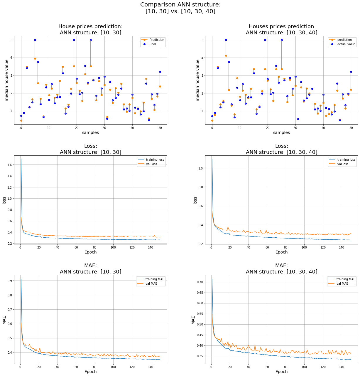
The last two models #
ns = 50 # number of samples to visualize
id_one, id_two = -2,-1 # index of the two models we want to compare

# Initialize the figure
width, height = 7, 10 # single pic
rows, columns = 3, 2
fig = plt.figure(figsize = (width*rows,height*columns))

idx_model = id_one
y_pred = pred_list[idx_model] # prediction of a certain model

## SBP 1
ax1 = fig.add_subplot(rows, columns, 1);
for i in range(0,ns+1):
    ax1.plot(i,y_pred[i], 'darkorange',marker='o')
    ax1.plot(i,y_test[i], 'b',marker='o')
    ax1.plot([i, i], [y_pred[i], y_test[i]], color='grey') # distance btw y_test and y_pred
ax1.legend(['Prediction','Real'])
ax1.set_xlabel('samples',fontsize=14);
ax1.set_ylabel('median house value',fontsize=14);
ax1.set_title(f'House prices prediction:\nANN structure: {net_struct[idx_model]}',fontsize=18);
ax1.grid(color='grey', linestyle='-', linewidth=0.5);

## SBP 3
ax3 = fig.add_subplot(rows, columns, 3);
ax3.plot(range(1,EPOCHS+1), training_loss[idx_model], label="training loss")
ax3.plot(range(1,EPOCHS+1), val_loss[idx_model], label="val loss")
ax3.legend()
ax3.set_xlabel('Epoch',fontsize=14);
ax3.set_ylabel('loss',fontsize=14);
ax3.set_title(f'Loss:\nANN structure: {net_struct[idx_model]}',fontsize=18);
ax3.grid(color='grey', linestyle='-', linewidth=0.5);

## SBP 5
ax5 = fig.add_subplot(rows, columns, 5);
ax5.plot(range(1,EPOCHS+1), training_MAE[idx_model], label="training MAE")
ax5.plot(range(1,EPOCHS+1), val_MAE[idx_model], label="val MAE")
ax5.legend()
ax5.set_xlabel('Epoch',fontsize=14);
ax5.set_ylabel('MAE',fontsize=14);
ax5.set_title(f'MAE:\nANN structure: {net_struct[idx_model]}',fontsize=18);
ax5.grid(color='grey', linestyle='-', linewidth=0.5);

idx_model = id_two
y_pred = pred_list[idx_model] # prediction of a certain model

## SBP 2
ax2 = fig.add_subplot(rows, columns, 2);
for i in range(0,ns+1):
    ax2.plot(i,y_pred[i], 'darkorange',marker='o')
    ax2.plot(i,y_test[i], 'b',marker='o')
    ax2.plot([i, i], [y_pred[i], y_test[i]], color='grey') # distance btw y_test and y_pred
ax2.legend(['prediction','actual value'])
ax2.set_xlabel('samples',fontsize=14);
ax2.set_ylabel('median house value',fontsize=14);
ax2.set_title(f'Houses prices prediction\nANN structure: {net_struct[idx_model]}',fontsize=18);
ax2.grid(color='grey', linestyle='-', linewidth=0.5);

## SBP 4
ax4 = fig.add_subplot(rows, columns, 4);
ax4.plot(range(1,EPOCHS+1), training_loss[idx_model], label="training loss")
ax4.plot(range(1,EPOCHS+1), val_loss[idx_model], label="val loss")
ax4.legend()
ax4.set_xlabel('Epoch',fontsize=14);
ax4.set_ylabel('loss',fontsize=14);
ax4.set_title(f'Loss:\nANN structure: {net_struct[idx_model]}',fontsize=18);
ax4.grid(color='grey', linestyle='-', linewidth=0.5);

## SBP 6
ax6 = fig.add_subplot(rows, columns, 6);
ax6.plot(range(1,EPOCHS+1), training_MAE[idx_model], label="training MAE")
ax6.plot(range(1,EPOCHS+1), val_MAE[idx_model], label="val MAE")
ax6.legend()
ax6.set_xlabel('Epoch',fontsize=14);
ax6.set_ylabel('MAE',fontsize=14);
ax6.set_title(f'MAE:\nANN structure: {net_struct[idx_model]}',fontsize=18);
ax6.grid(color='grey', linestyle='-', linewidth=0.5);

# set the spacing between subplots
plt.suptitle(f"Comparison ANN structure:\n{net_struct[id_one]} vs. {net_struct[id_two]}", fontsize=20)
plt.subplots_adjust(top=0.9,
                    wspace=0.25,
                    hspace=0.35)

plt.show()